23 Performance Optimization

Profiling R code, vectorization strategies, memory-efficient history storage, and when to consider Rcpp — demonstrated on game-theory simulations.

Learning objectives

• Profile R code using system.time() and manual benchmarking to identify bottlenecks.
• Replace explicit loops with vectorized matrix operations for payoff computation.
• Pre-allocate data structures to avoid the performance cost of growing objects.
• Recognize when Rcpp would provide further speedups and describe the conceptual approach.

23.1 Motivation

A single run of the Axelrod tournament (18) with eight strategies and 200 rounds finishes in under a second. But scale the problem — 100 strategies, 1000 rounds, spatial grids of 10,000 agents, evolutionary dynamics over 500 generations — and naive R code can take hours. The difference between a simulation that runs in 30 seconds and one that runs in 30 minutes is often not a better algorithm, but better use of R’s strengths.

R is slow when you fight it: growing vectors with c(), appending rows with rbind(), nested loops over scalar operations. R is fast when you work with it: pre-allocated matrices, vectorized arithmetic, and functions that call optimized C code under the hood. In this chapter, we profile a game-theory simulation, identify the bottlenecks, and eliminate them.

23.2 Theory

23.2.1 Why R loops are slow

R is an interpreted language with dynamic typing. Each iteration of a for loop involves type checking, memory allocation, and function dispatch. A loop that runs \(n\) times incurs this overhead \(n\) times. Vectorized operations like A %*% x delegate the loop to compiled C or Fortran code, paying the overhead once and executing the loop at native speed.

23.2.2 Three levels of optimization

1. Vectorization: Replace element-wise loops with matrix operations. This is always the first step and often delivers 10–100x speedups.
2. Memory pre-allocation: Replace c(vec, new_val) and rbind(df, new_row) with indexed assignment into pre-allocated objects. Growing objects forces R to copy the entire object on each append.
3. Compiled code (Rcpp): For algorithms that cannot be vectorized — complex conditional logic, recursive data structures, sequential dependencies — Rcpp lets you write inner loops in C++ while keeping the R interface. This is the tool of last resort, not the first.

23.2.3 The profiling workflow

1. Measure: Use system.time() to get elapsed time.
2. Identify: Find the hotspot — the innermost loop consuming most runtime.
3. Optimize: Apply vectorization, pre-allocation, or Rcpp.
4. Verify: Confirm the optimized code produces identical results.

23.3 Implementation in R

23.3.1 The baseline: loop-based spatial PD

We implement a simplified spatial Prisoner’s Dilemma on a grid, similar to 19. This is our baseline for optimization.

spatial_pd_loop <- function(n = 30, rounds = 50, b = 1.8) {
  grid <- matrix(sample(c(1L, 0L), n * n, replace = TRUE), nrow = n, ncol = n)

  # Store cooperation history
  coop_history <- numeric(rounds)

  for (t in seq_len(rounds)) {
    coop_history[t] <- mean(grid)

    # Compute payoffs (loop version)
    payoffs <- matrix(0, nrow = n, ncol = n)
    for (i in seq_len(n)) {
      for (j in seq_len(n)) {
        # Four neighbors with periodic boundary
        neighbors <- list(
          c(((i - 2) %% n) + 1, j),
          c((i %% n) + 1, j),
          c(i, ((j - 2) %% n) + 1),
          c(i, (j %% n) + 1)
        )
        for (nb in neighbors) {
          ni <- nb[1]; nj <- nb[2]
          # PD payoff: C vs C = 1, C vs D = 0, D vs C = b, D vs D = 0
          if (grid[i, j] == 1L && grid[ni, nj] == 1L) {
            payoffs[i, j] <- payoffs[i, j] + 1
          } else if (grid[i, j] == 0L && grid[ni, nj] == 1L) {
            payoffs[i, j] <- payoffs[i, j] + b
          }
        }
      }
    }

    # Imitation: copy highest-earning neighbor or self
    new_grid <- grid
    for (i in seq_len(n)) {
      for (j in seq_len(n)) {
        best_payoff <- payoffs[i, j]
        best_strategy <- grid[i, j]
        neighbors <- list(
          c(((i - 2) %% n) + 1, j),
          c((i %% n) + 1, j),
          c(i, ((j - 2) %% n) + 1),
          c(i, (j %% n) + 1)
        )
        for (nb in neighbors) {
          ni <- nb[1]; nj <- nb[2]
          if (payoffs[ni, nj] > best_payoff) {
            best_payoff <- payoffs[ni, nj]
            best_strategy <- grid[ni, nj]
          }
        }
        new_grid[i, j] <- best_strategy
      }
    }
    grid <- new_grid
  }

  coop_history
}

23.3.2 The optimized version: vectorized spatial PD

The key insight is that summing neighbor cooperators is a convolution — shifting the grid in each direction and adding. We replace the inner double loops with matrix shifts.

# Helper: shift a matrix with periodic boundaries
shift_matrix <- function(mat, row_shift, col_shift) {
  n <- nrow(mat)
  rows <- ((seq_len(n) - 1 + row_shift) %% n) + 1
  cols <- ((seq_len(n) - 1 + col_shift) %% n) + 1
  mat[rows, cols]
}

# Vectorized spatial PD simulation
spatial_pd_vectorized <- function(n = 30, rounds = 50, b = 1.8) {
  grid <- matrix(sample(c(1L, 0L), n * n, replace = TRUE), nrow = n, ncol = n)
  coop_history <- numeric(rounds)

  for (t in seq_len(rounds)) {
    coop_history[t] <- mean(grid)

    # Count cooperating neighbors (vectorized)
    coop_neighbors <- shift_matrix(grid, -1, 0) +
                      shift_matrix(grid, 1, 0) +
                      shift_matrix(grid, 0, -1) +
                      shift_matrix(grid, 0, 1)

    # Payoffs: cooperators get 1 per cooperating neighbor
    #          defectors get b per cooperating neighbor
    payoffs <- ifelse(grid == 1L, coop_neighbors, b * coop_neighbors)

    # Imitation: compare with all neighbors' payoffs
    best_payoff <- payoffs
    best_strategy <- grid

    for (shift in list(c(-1,0), c(1,0), c(0,-1), c(0,1))) {
      nb_payoff <- shift_matrix(payoffs, shift[1], shift[2])
      nb_strategy <- shift_matrix(grid, shift[1], shift[2])
      update <- nb_payoff > best_payoff
      best_payoff[update] <- nb_payoff[update]
      best_strategy[update] <- nb_strategy[update]
    }

    grid <- best_strategy
  }

  coop_history
}

23.3.3 Benchmarking the two implementations

# Manual benchmarking function
benchmark_fn <- function(fn, ..., n_reps = 5) {
  times <- numeric(n_reps)
  for (i in seq_len(n_reps)) {
    set.seed(42)
    times[i] <- system.time(fn(...))["elapsed"]
  }
  list(mean = mean(times), sd = sd(times), times = times)
}

cat("Benchmarking spatial PD (30x30 grid, 50 rounds)...\n\n")

#> Benchmarking spatial PD (30x30 grid, 50 rounds)...

time_loop <- benchmark_fn(spatial_pd_loop, n = 30, rounds = 50)
time_vec  <- benchmark_fn(spatial_pd_vectorized, n = 30, rounds = 50)

cat(sprintf("  Loop-based:  %.3f s (sd: %.3f)\n", time_loop$mean, time_loop$sd))

#>   Loop-based:  0.266 s (sd: 0.021)

cat(sprintf("  Vectorized:  %.3f s (sd: %.3f)\n", time_vec$mean, time_vec$sd))

#>   Vectorized:  0.016 s (sd: 0.010)

cat(sprintf("  Speedup:     %.1fx\n", time_loop$mean / time_vec$mean))

#>   Speedup:     16.6x

23.3.4 Verifying correctness

set.seed(42)
result_loop <- spatial_pd_loop(n = 20, rounds = 30)
set.seed(42)
result_vec <- spatial_pd_vectorized(n = 20, rounds = 30)

cat("Verification: loop vs vectorized produce identical results:\n")

#> Verification: loop vs vectorized produce identical results:

cat(sprintf("  Max absolute difference: %.10f\n", max(abs(result_loop - result_vec))))

#>   Max absolute difference: 0.0000000000

cat(sprintf("  All equal: %s\n", all.equal(result_loop, result_vec)))

#>   All equal: TRUE

23.3.5 Visualizing the benchmark

bench_df <- tibble(
  implementation = c("Loop-based", "Vectorized"),
  mean_time = c(time_loop$mean, time_vec$mean),
  sd_time = c(time_loop$sd, time_vec$sd)
) |>
  mutate(implementation = factor(implementation,
                                  levels = c("Loop-based", "Vectorized")))

p_bench <- ggplot(bench_df, aes(x = implementation, y = mean_time,
                                 fill = implementation)) +
  geom_col(width = 0.6) +
  geom_errorbar(aes(ymin = pmax(mean_time - sd_time, 0),
                    ymax = mean_time + sd_time),
                width = 0.15) +
  geom_text(aes(label = sprintf("%.3fs", mean_time)),
            vjust = -0.5, size = 3.5) +
  scale_fill_manual(values = c("Loop-based" = okabe_ito[6],
                                "Vectorized" = okabe_ito[3])) +
  theme_publication() +
  theme(legend.position = "none") +
  labs(title = "Spatial PD: Loop vs Vectorized",
       x = NULL, y = "Execution time (seconds)")

p_bench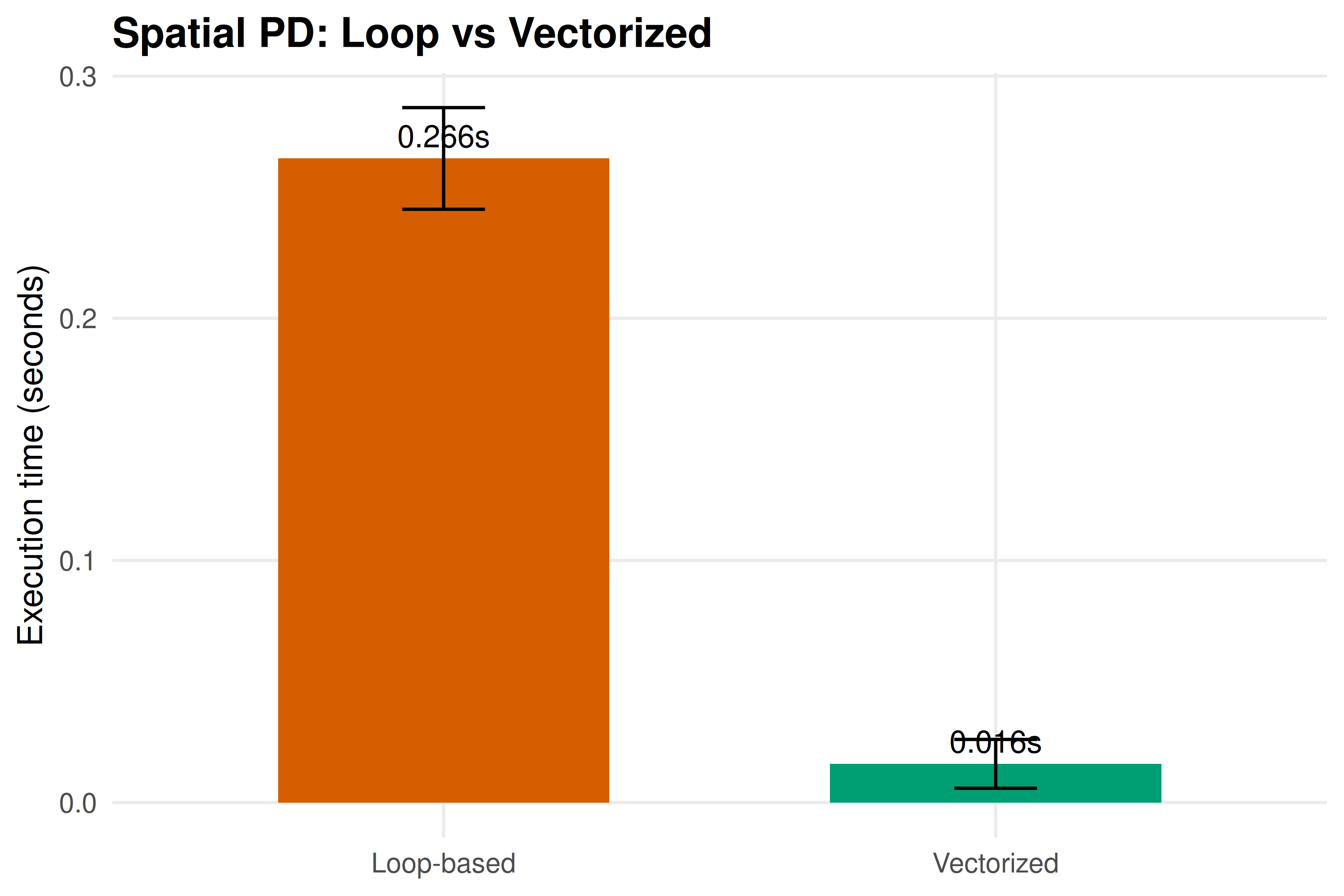

Figure 23.1: Execution time comparison for the spatial Prisoner’s Dilemma simulation. Vectorized matrix operations eliminate the inner double loops, achieving a substantial speedup over the naive loop-based implementation.

save_pub_fig(p_bench, "performance-comparison", width = 6, height = 4)

23.3.6 Scaling behavior

How does each implementation scale with grid size?

grid_sizes <- c(10, 15, 20, 30, 40, 50)
scaling_results <- list()

for (n in grid_sizes) {
  set.seed(42)
  t_loop <- system.time(spatial_pd_loop(n = n, rounds = 20))["elapsed"]
  set.seed(42)
  t_vec <- system.time(spatial_pd_vectorized(n = n, rounds = 20))["elapsed"]
  scaling_results[[length(scaling_results) + 1]] <- tibble(
    grid_size = n,
    n_cells = n^2,
    loop_time = t_loop,
    vec_time = t_vec
  )
}

scaling_df <- bind_rows(scaling_results) |>
  pivot_longer(cols = c(loop_time, vec_time),
               names_to = "method", values_to = "time") |>
  mutate(method = ifelse(method == "loop_time", "Loop-based", "Vectorized"))

p_scaling <- ggplot(scaling_df, aes(x = n_cells, y = time, colour = method)) +
  geom_point(size = 2.5) +
  geom_line(linewidth = 0.8) +
  scale_x_log10(labels = scales::comma_format()) +
  scale_y_log10(labels = scales::label_number(suffix = "s")) +
  scale_colour_manual(values = c("Loop-based" = okabe_ito[6],
                                  "Vectorized" = okabe_ito[3]),
                      name = "Implementation") +
  annotation_logticks(sides = "bl") +
  theme_publication() +
  labs(title = "Scaling: Time vs Grid Size (log-log)",
       x = "Number of cells", y = "Execution time")

p_scaling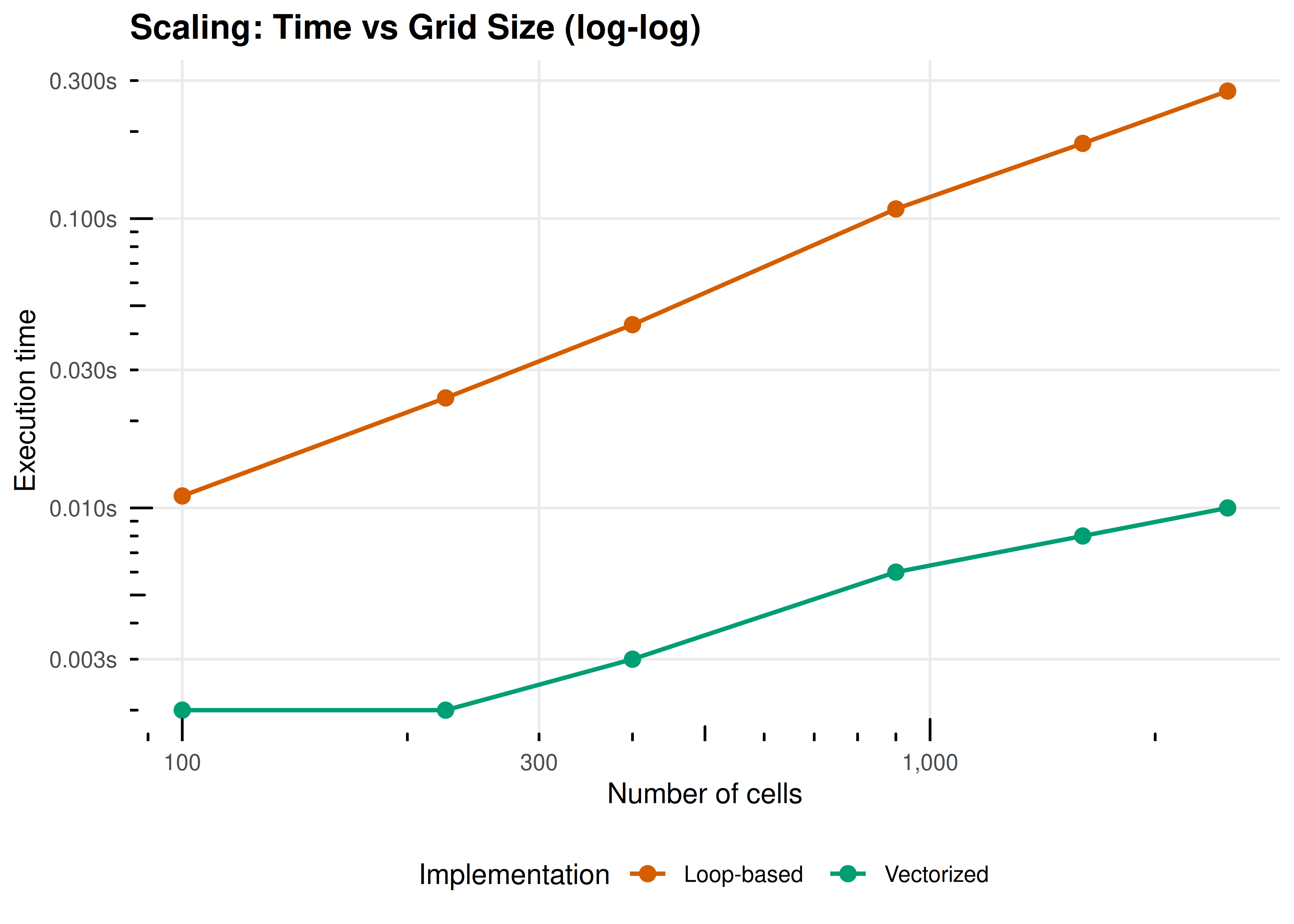

Figure 23.2: Scaling behavior of loop-based vs vectorized spatial PD as grid size increases (fixed at 20 rounds). Both scale roughly quadratically in the number of cells (as expected for a grid simulation), but the vectorized version maintains a consistent advantage. The log-log plot reveals parallel scaling slopes with a constant multiplicative gap.

save_pub_fig(p_scaling, "performance-scaling", width = 7, height = 5)

23.4 Worked example

We optimize the spatial PD simulation step by step, measuring the impact of each change.

23.4.1 Step 1: Profile the baseline

cat("Profiling the loop-based implementation (40x40, 20 rounds):\n\n")

#> Profiling the loop-based implementation (40x40, 20 rounds):

set.seed(42)
t_full <- system.time({
  result_full <- spatial_pd_loop(n = 40, rounds = 20)
})
cat(sprintf("  Total elapsed time: %.3f s\n", t_full["elapsed"]))

#>   Total elapsed time: 0.176 s

cat("  Bottleneck: nested loops over all cells and neighbors for payoff computation.\n")

#>   Bottleneck: nested loops over all cells and neighbors for payoff computation.

cat("  Each round iterates over n^2 cells x 4 neighbors = 6,400 scalar operations.\n")

#>   Each round iterates over n^2 cells x 4 neighbors = 6,400 scalar operations.

cat("  Over 20 rounds: 128,000 individual loop iterations.\n")

#>   Over 20 rounds: 128,000 individual loop iterations.

23.4.2 Step 2: Vectorize payoff computation

The key rewrite replaces the inner double loop with four matrix-shift operations.

set.seed(42)
t_vec <- system.time(result_vec <- spatial_pd_vectorized(n = 40, rounds = 20))
cat(sprintf("  Vectorized time:  %.3f s\n", t_vec["elapsed"]))

#>   Vectorized time:  0.006 s

cat(sprintf("  Loop-based time:  %.3f s\n", t_full["elapsed"]))

#>   Loop-based time:  0.176 s

cat(sprintf("  Speedup:          %.1fx\n", t_full["elapsed"] / t_vec["elapsed"]))

#>   Speedup:          29.3x

23.4.3 Step 3: Memory pre-allocation matters

A common anti-pattern in R is growing a data frame row by row. We demonstrate the cost.

# Growing a vector vs pre-allocated
grow_vector <- function(n) {
  v <- c()
  for (i in seq_len(n)) {
    v <- c(v, i)
  }
  v
}

prealloc_vector <- function(n) {
  v <- numeric(n)
  for (i in seq_len(n)) {
    v[i] <- i
  }
  v
}

sizes <- c(1000, 5000, 10000, 20000)
prealloc_results <- list()

for (sz in sizes) {
  t_grow <- system.time(grow_vector(sz))["elapsed"]
  t_pre <- system.time(prealloc_vector(sz))["elapsed"]
  prealloc_results[[length(prealloc_results) + 1]] <- tibble(
    n = sz, grow = t_grow, prealloc = t_pre
  )
}

prealloc_df <- bind_rows(prealloc_results)

cat("Growing vs pre-allocated vector (seconds):\n\n")

#> Growing vs pre-allocated vector (seconds):

cat(sprintf("  %-8s  %-8s  %-10s  %s\n", "n", "Grow", "Prealloc", "Speedup"))

#>   n         Grow      Prealloc    Speedup

for (i in seq_len(nrow(prealloc_df))) {
  sp <- if (prealloc_df$prealloc[i] > 0) prealloc_df$grow[i]/prealloc_df$prealloc[i] else Inf
  cat(sprintf("  %-8s  %-8.4f  %-10.4f  %.0fx\n",
              scales::comma(prealloc_df$n[i]), prealloc_df$grow[i], prealloc_df$prealloc[i], sp))
}

#>   1,000     0.0040    0.0030      1x
#>   5,000     0.0220    0.0010      22x
#>   10,000    0.0860    0.0000      Infx
#>   20,000    0.3350    0.0010      335x

The growing vector copies the entire vector on each append, producing \(O(n^2)\) total work. Pre-allocation is \(O(n)\).

23.4.4 When to consider Rcpp

For the spatial PD, vectorization delivered a large speedup because the core operation — summing neighbor states — is naturally expressed as matrix arithmetic. But some algorithms resist vectorization:

• Sequential dependencies: When round \(t\)’s outcome depends on the order of updates within round \(t-1\), you cannot compute all cells simultaneously.
• Complex conditionals: Strategies with multi-step memory require per-agent branching that ifelse() cannot cleanly express.
• Graph traversal: Shortest paths and clustering on irregular networks involve queues and visited-node tracking that are inherently sequential.

In these cases, Rcpp lets you write the inner loop in C++ while keeping the R interface. A typical C++ function takes R matrices as input, performs the sequential computation, and returns the result — with 50–200x speedups over R loops.

The decision rule is simple: vectorize first, Rcpp second. If the bottleneck can be expressed as matrix operations, do that. Only reach for Rcpp when it cannot.

23.5 Extensions

• Parallel computation: R’s parallel package provides mclapply() (Unix) and parLapply() (all platforms) for embarrassingly parallel tasks like running independent replications.
• Sparse matrices: The Matrix package provides sparse representations that reduce storage from \(O(n^2)\) to \(O(m)\) for networks with \(m\) edges, and its arithmetic skips zero entries.
• Byte compilation: compiler::cmpfun() byte-compiles R functions, delivering 2–5x speedups for loop-heavy code with zero code changes.
• Profiling tools: Rprof() provides sampling-based profiling, and profvis::profvis() offers interactive flame-graph visualizations for identifying hotspots.

Exercises

1. Vectorize the tournament. The run_tournament() function in R/axelrod.R uses nested loops over strategy pairs. Each match is independent, so the outer loop is embarrassingly parallel. Write a version that stores results in a pre-allocated matrix and measure the speedup.

2. Memory scaling. Modify the spatial PD to store the full grid at each round using (a) a growing list grid_list[[t]] <- grid and (b) a pre-allocated 3D array array(0L, dim = c(n, n, rounds)). Benchmark both for \(n = 50\) and 100 rounds.

3. Identify the crossover. Find the grid size \(n\) at which the vectorized version becomes faster than the loop-based version. Plot both timing curves and mark the crossover point.

Solutions appear in D.

This book was built by the bookdown R package.