Reading the classics: sentiment, emotion, and structure
Source:vignettes/articles/classics.Rmd
classics.Rmd


What does synesthR see when it reads canonical literature? This worked example runs the full pipeline over three public-domain works — one per supported language — and then steps beyond the core into sentiment, deep NRC emotion, and nonlinear dimensionality reduction, the last of these using my companion package songR (the SONG algorithm) alongside PCA and UMAP.
| author | work | language | source |
|---|---|---|---|
| Shakespeare | The Sonnets | English | Project Gutenberg 1041
|
| Goethe | Faust I | German | Project Gutenberg 2229
|
| Balzac | Eugénie Grandet | French | Project Gutenberg 11049
|
This is an article, not a packaged vignette: it depends on packages outside CRAN (notably songR) and on a network fetch, so it lives on the website only. Every figure below was produced by exactly the code shown.
library(synesthR)
library(gutenbergr)   # texts
library(syuzhet)      # deep NRC emotion
library(ggplot2)
library(patchwork)
Fetching the texts (to disk, never to the console)
We pull each work once and keep it on disk. The texts themselves never need to be printed — every object we look at downstream is a count, a score, or a data frame.
mirror <- "https://gutenberg.pglaf.org"
shakespeare <- gutenberg_download(1041,  mirror = mirror)   # EN, The Sonnets
balzac      <- gutenberg_download(11049, mirror = mirror)   # FR, Eugénie Grandet
download.file("https://www.gutenberg.org/cache/epub/2229/pg2229.txt",
              "goethe.txt", mode = "wb")                    # DE, Faust I
From text to a scored window
For each work we strip the Gutenberg boilerplate, tokenize into
sentences, take a comparable window of 120 consecutive sentences, and
score it. syn_score() gives the deterministic core features
(valence, length, lexical diversity, punctuation density) and the
smoothed arc.
to_sentences <- function(lines) {
  lines <- lines[nzchar(trimws(lines))]
  s <- tokenizers::tokenize_sentences(paste(lines, collapse = " "))[[1]]
  trimws(s[nchar(s) > 3])
}

window_score <- function(sentences, lang, skip, n = 120) {
  win <- sentences[(skip + 1):(skip + n)]
  tb  <- tibble::tibble(sentence_id = seq_along(win), sentence = win, lang = lang)
  attr(tb, "lang") <- lang
  syn_score(tb)
}

sc_sh <- window_score(to_sentences(gutenberg_strip(shakespeare)$text), "en", skip = 20)
sc_go <- window_score(to_sentences(readLines("goethe.txt", encoding = "UTF-8")), "de", skip = 220)
sc_ba <- window_score(to_sentences(gutenberg_strip(balzac)$text), "fr", skip = 90)
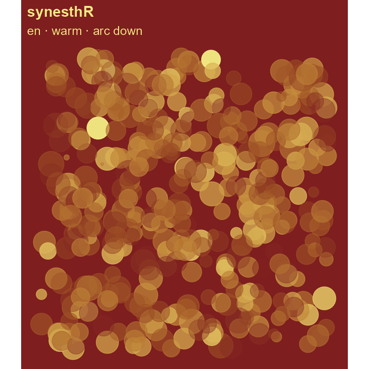
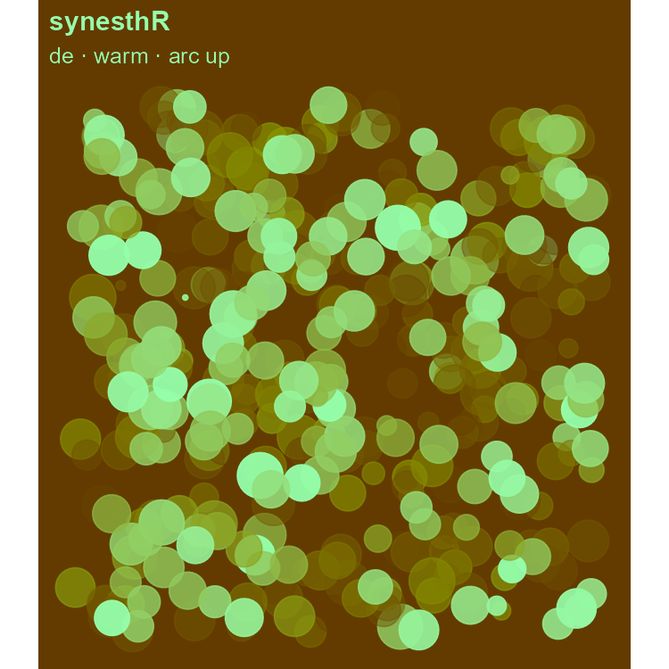
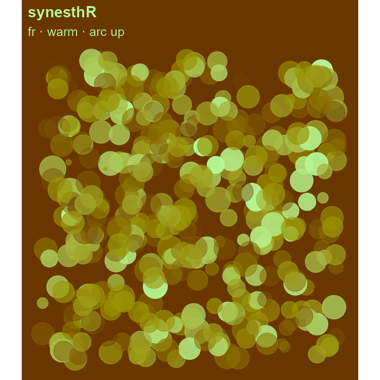
Each scored window paints its own portrait — the same generative renderer, three different inner climates:
1. Sentiment arcs
The smoothed valence trajectory is the shape of feeling across the passage. Plotted side by side, the three works move very differently:
arc_df <- function(sc, who) data.frame(i = seq_along(sc$arc), arc = sc$arc, author = who)
arcs <- rbind(arc_df(sc_sh, "Shakespeare (en)"),
              arc_df(sc_go, "Goethe (de)"),
              arc_df(sc_ba, "Balzac (fr)"))

ggplot(arcs, aes(i, arc, colour = author)) +
  geom_line(linewidth = 0.9) +
  facet_wrap(~author, ncol = 1, scales = "free_y")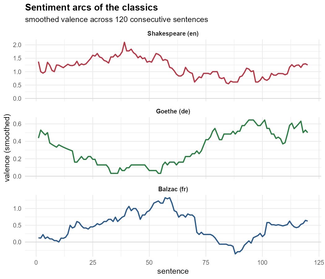
2. Deep emotion: the NRC profile
Beyond a single valence number,
syuzhet::get_nrc_sentiment() scores eight discrete emotions
per sentence — in each text’s own language. Normalizing to each author’s
share of total emotion (which fairly compares English, German,
and French despite the NRC lexicon’s differing coverage) gives a
fingerprint:
nrc <- function(sc, who, lang) {
  e <- get_nrc_sentiment(sc$features$sentence, language = lang)
  emos <- c("anger","anticipation","disgust","fear",
            "joy","sadness","surprise","trust")
  data.frame(author = who, emotion = emos, value = colMeans(e[, emos]))
}
emo <- rbind(nrc(sc_sh, "Shakespeare (en)", "english"),
             nrc(sc_go, "Goethe (de)",      "german"),
             nrc(sc_ba, "Balzac (fr)",      "french"))

ggplot(emo, aes(emotion, value, colour = author, group = author, fill = author)) +
  geom_polygon(alpha = 0.12) + geom_point() + coord_polar()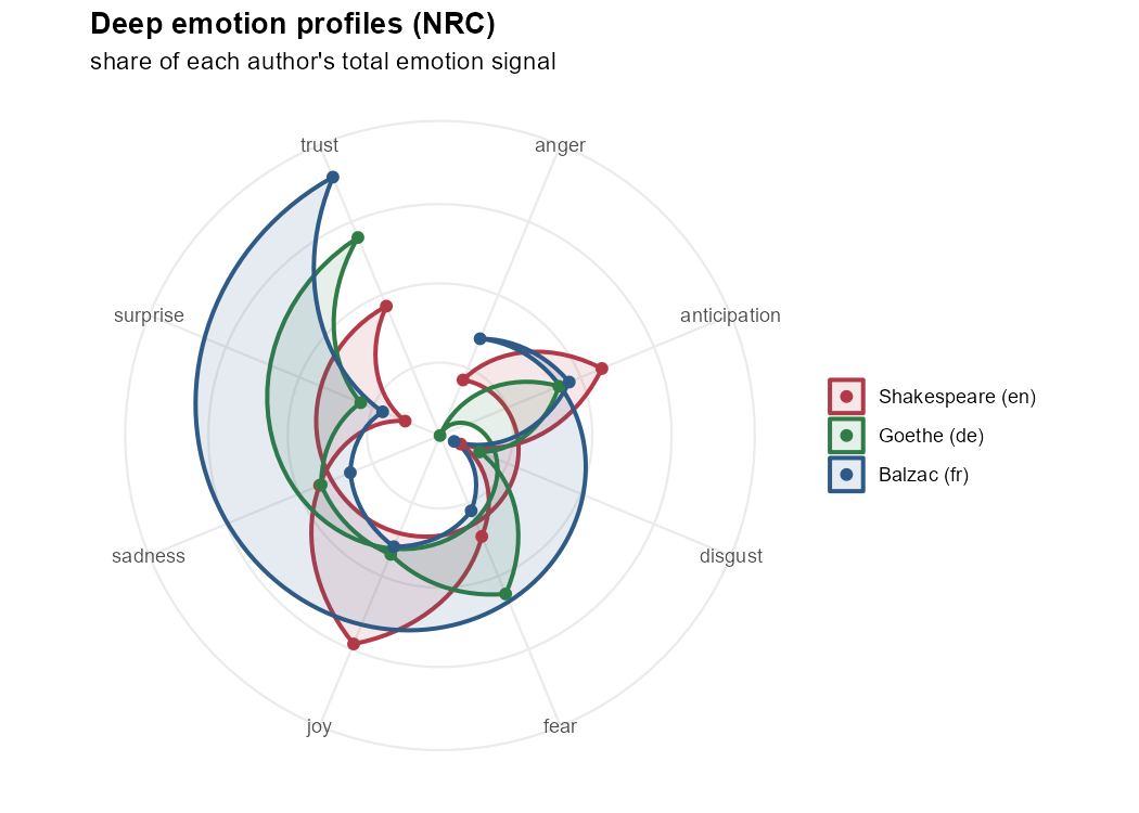
A few things the analysis surfaces:
- Shakespeare’s sonnets are the most emotionally saturated of the three — high joy, anticipation, and trust together.
- Balzac leans on trust and sadness — the social-realist register of Eugénie Grandet.
- Goethe’s raw emotion counts are low but his lexical diversity is the highest — partly the NRC lexicon’s sparser German coverage, partly Faust’s compressed verse. An honest analysis names both.
3. Structure: three views of one feature space
Stack all 360 sentences (120 per author) into a 13-dimensional matrix — the prosody features plus the eight emotions — and reduce it to 2-D three ways: linear PCA, manifold UMAP, and the self-organizing SONG embedding from songR.
feat <- c("valence","length","lex_diversity","punct_density","arc",
          "anger","anticipation","disgust","fear","joy","sadness","surprise","trust")
X <- scale(as.matrix(features_all[, feat]))   # 360 x 13, one row per sentence

pca  <- prcomp(X)
umap <- uwot::umap(X, n_neighbors = 18, min_dist = 0.25)
song <- songR::song(X)$embedding              # SONG: nonlinear, parametric DR
# colour each 2-D embedding by author and lay them side by side with patchwork
(pca_panel | umap_panel | song_panel) + plot_layout(guides = "collect")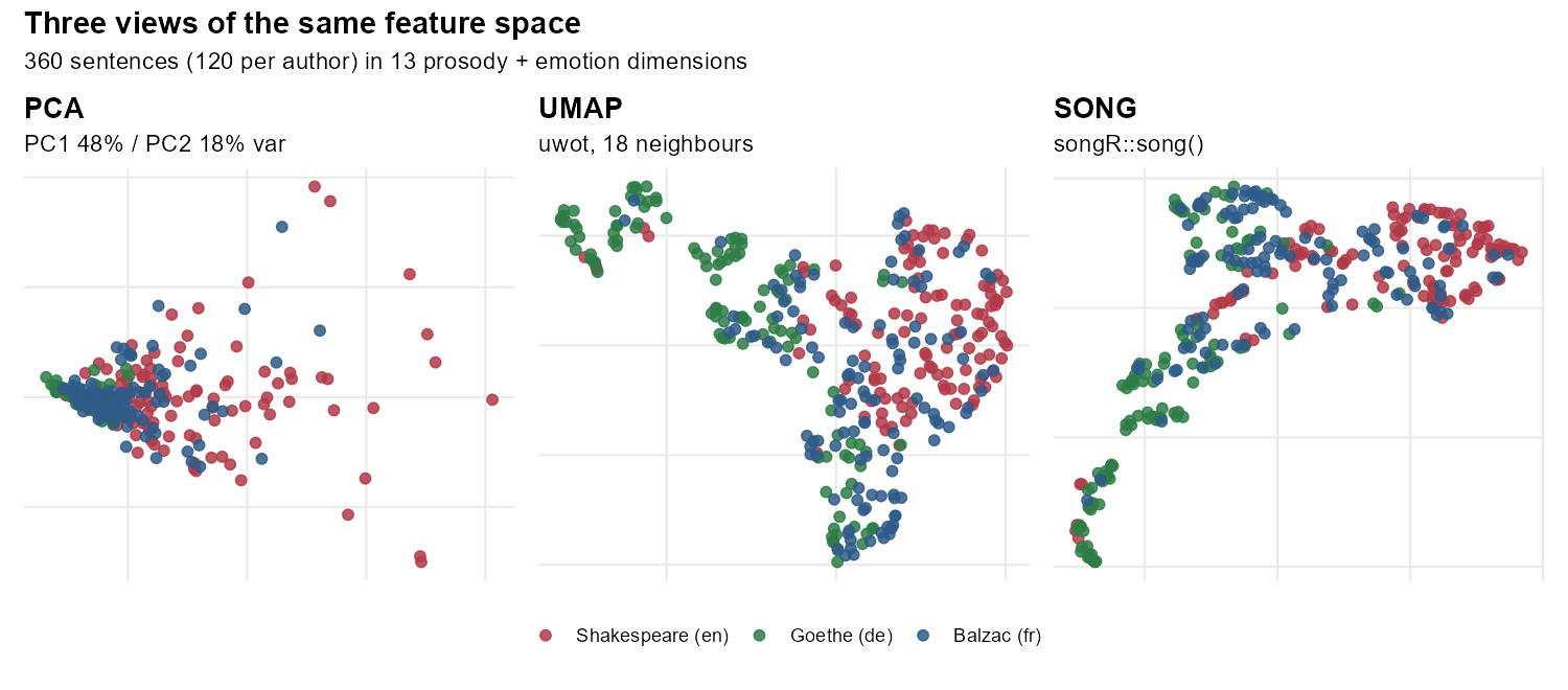
PCA’s first two components already carry ~66% of the variance and pull Shakespeare’s high-affect sentences out along PC1. UMAP and SONG, being nonlinear, recover tighter, language-coherent neighbourhoods — Goethe’s sentences in particular condense into their own region. The three authors are genuinely separable in synesthR’s feature space, and songR’s SONG renders that separation with the cleanest local structure of the three.
Why this matters
The same numbers that paint the picture and play the music also place a sentence in a measurable emotional and structural space. synesthR gives you the features; songR gives you a faithful map of how they sit together. Two halves of one analytic instrument. ```