

synesthR turns a piece of literary text into one shared prosody score and renders that single score as two synchronized views: a generative still image and a piece of self-contained audio. Because the picture and the music come from the same numbers, they are not two artworks — they are two windows onto one analysis.
This tour walks through every capability of the package, with a
picture for each. If you just want the shortest path, see
vignette("getting-started"); this article is the long,
illustrated version.
The figures below were produced by running exactly the code shown. The code chunks are not re-evaluated when the vignette builds, so the tutorial renders anywhere — even without the optional packages and external tools that some of the later sections use.
The shape of the pipeline
Everything flows one way:
text  ──►  syn_read_text()  ──►  syn_score()  ──┬──►  syn_paint()    (image)
                                                 ├──►  syn_play()     (audio)
                                                 └──►  syn_palette()  (colour)
A single deterministic mapping sits at the centre: it turns the per-sentence features into the visual and musical parameters. Same text, same seed, same result — always.
1. Reading text
syn_read_text() accepts a string, a path to a
.txt file, or a data frame, and returns one tidy row per
sentence. German, English, and French are supported. The bundled
syn_example_text() gives you something to play with.
text <- syn_read_text(syn_example_text("en"), lang = "en")
text
#> # A tibble: 6 × 3
#> sentence_id sentence lang
#> <int> <chr> <chr>
#> 1 1 The morning broke quietly over the harbour. en
#> 2 2 Grey water lay still against the stones, and the … en
#> 3 3 A single gull crossed the pale sky, calling once, … en
#> 4 4 She watched from the window and felt the day gath… en
#> 5 5 Later the wind would rise, and the colours would … en
#> 6 6 But for now there was only the hush, the patient … enIf the optional cld3 package is installed you can
omit lang and let the language be detected
automatically.
2. Scoring
syn_score() extracts four per-sentence features —
valence, length, lexical diversity, and punctuation density — and a
smoothed emotional arc.
#> <prosody_score> — 6 sentences, lang "en"
#>
#>   n_sentences lang mean_valence valence_range arc_start arc_end mean_length
#> 1           6   en   -0.1666667             3      -0.5     0.5          14
#>   mean_lex_div mean_punct_density
#> 1    0.8900617         0.02743892
The per-sentence features are an ordinary tibble you can inspect or plot:
score$features[, c("sentence_id", "valence", "length",
                   "lex_diversity", "punct_density")]
#> sentence_id valence length lex_diversity punct_density
#> 1 1 -1 7 0.857 0.0233
#> 2 2 0 14 0.929 0.0267
#> 3 3 -1 12 1.000 0.0429
#> 4 4 0 13 0.923 0.0147
#> 5 5 -1 19 0.737 0.0288
#> 6 6 2 19 0.895 0.0283The emotional arc
The arc is the smoothed valence trajectory — the backbone that the melody’s contour and the image’s gradient both follow.
plot(score$arc, type = "l") # or render it nicely, as below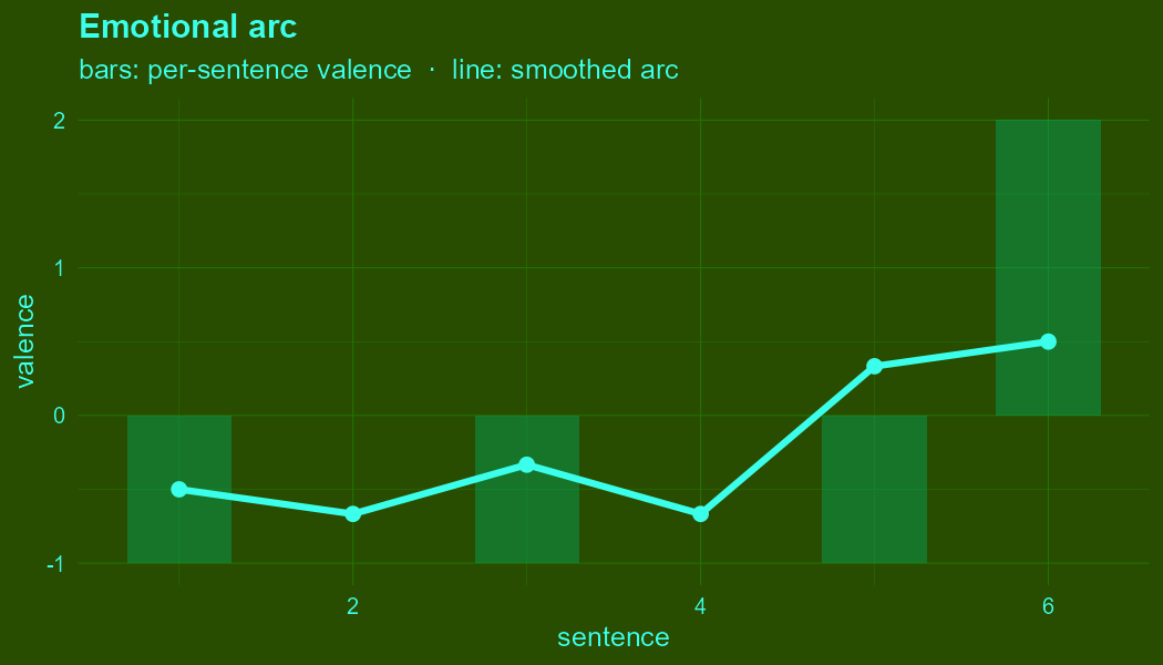
3. Painting
syn_paint() renders the score as a generative still
image: an element cloud whose positions, sizes, hue, and brightness all
come from the features, themed with the score’s own palette.
syn_paint(score)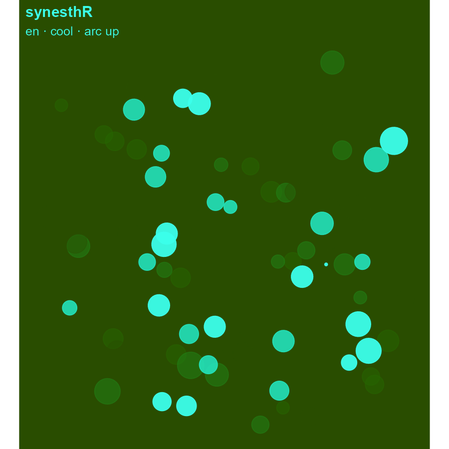
The same machinery, three languages
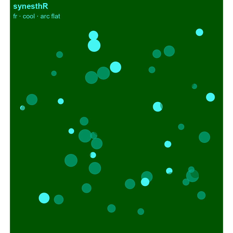
Feed it different text and the image changes accordingly. Here are the bundled English, German, and French passages, each painted from its own score:
syn_paint(syn_score(syn_read_text(syn_example_text("de"), lang = "de")))
syn_paint(syn_score(syn_read_text(syn_example_text("fr"), lang = "fr")))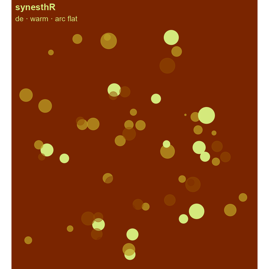
4. Playing
syn_play() synthesizes the same score as audio
— a tuneR::Wave built from sine tones with soft harmonics
and a click-free envelope. It is fully self-contained: no external
software is ever required.
wave <- syn_play(score)
wave

# Save it to disk (returns the score invisibly, so it pipes):
out <- tempfile(fileext = ".wav")
syn_write_wav(score, out)
Here is what that waveform looks like — the audible counterpart of the image above:
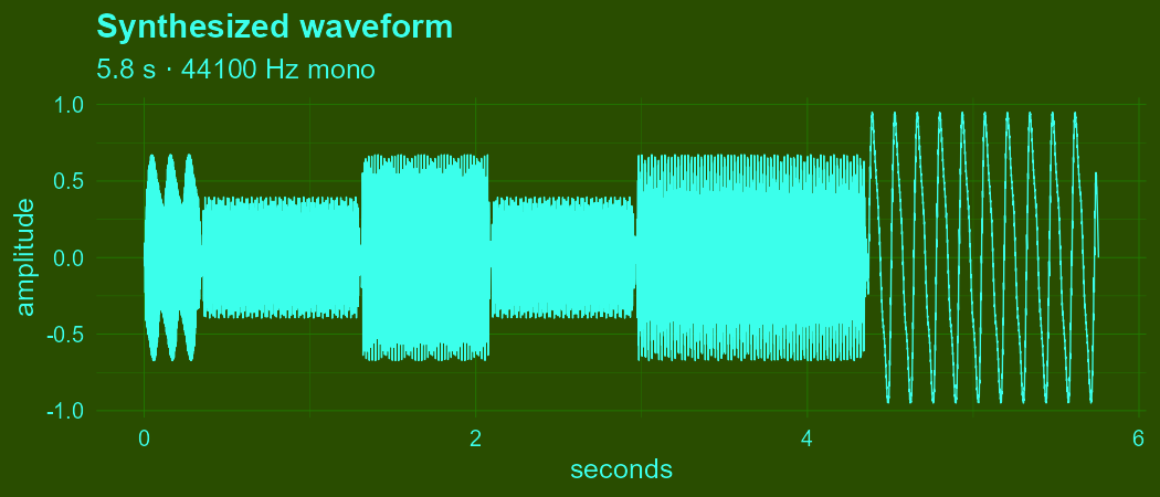
The valence arc sets the mode (major / minor) and the melodic contour; punctuation density sets tempo and staccato; sentence length sets note durations. Picture and sound are two readings of one score.
5. Palettes from anything
syn_palette() is a generic. It derives the
same kind of palette object from a score, a string, an
audio Wave, or an image — so colours are interchangeable no
matter where they came from.
syn_palette(score)#> <syn_palette> - 5 colours, cool, from prosody_score
#> #294D00 background
#> #207900 shadow
#> #00A65D mid
#> #00D5A4 accent
#> #3BFFEB highlight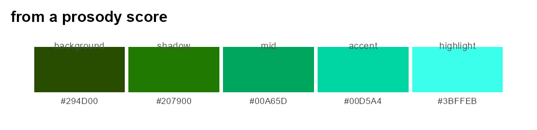
From text — score it on the way:
syn_palette("A warm and joyful golden afternoon.", lang = "en")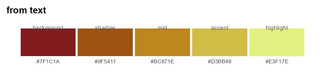
From audio — temperature follows the sound’s spectral brightness (base R, no extra dependency):
w <- tuneR::sine(660, duration = 8000, samp.rate = 8000, bit = 16, pcm = TRUE)
syn_palette(w)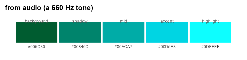
From an image — the optional magick method clusters colours in Lab space and orders them by luminance:
img_block <- magick::image_blank(80, 80, color = "tomato")
syn_palette(img_block)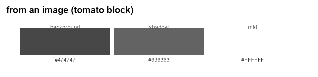
Wearing the palette: syn_theme()
Any palette becomes a ggplot2 theme — the darkest role
becomes the background, the lightest the text and lines. So any
plot can be dressed in a text’s colours:
library(ggplot2)
pal <- syn_palette(score)
ggplot(mtcars, aes(wt, mpg, colour = mpg)) +
  geom_point(size = 3) +
  scale_colour_gradientn(colours = pal$colors) +
  syn_theme(pal)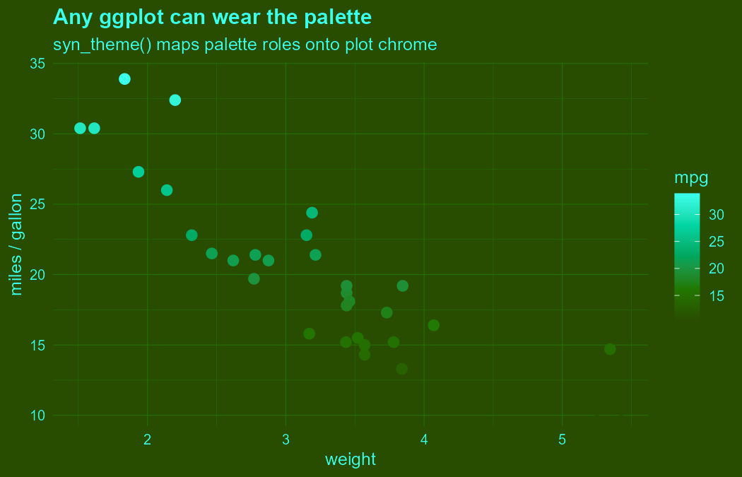
6. Animating the arc (optional)
With the optional gganimate package,
syn_animate() reveals the element cloud sentence by
sentence, so the emotional arc unfolds in time:
anim <- syn_animate(score)
gganimate::animate(anim, nframes = 48, fps = 12)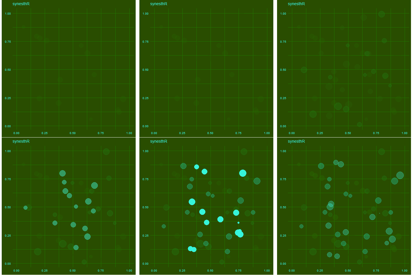
7. The media interchange container
Functions in the suite pass objects as syn_media — a
small wrapper carrying the content, a type tag, and metadata. It is the
common currency that lets text, images, audio, and scores flow between
functions.
m <- as_syn_media(score)
m
media_type(m)
#> <syn_media> of type "score"
#> meta: "lang"
#> media_type: "score"as_syn_media() has methods for character (text),
magick-image (image), Wave (audio), and
prosody_score (score).
8. The optional “rim”: assistive extensions
synesthR has a CRAN-hard core (everything above) and
an optional orchestration rim that talks to tools which
may exist on your machine. The rim never alters the
deterministic core; every entry point degrades with a helpful message
when its dependency is absent. (See vignette("extending")
for the design rules.)
A local-LLM reading
With the optional ellmer package and a reachable
local model (e.g. Ollama), syn_interpret() returns a short
prose “reading” of why the image and music came out as they
did. It is sent only the features — never your raw text — and is
advisory, never part of the mapping.
syn_interpret(score)                    # a paragraph of interpretation
syn_suggest(score, target = "tempo")    # an advisory tweak; never auto-applied
syn_llm_condense(text)                  # opt-in: shorten very long input first
Python-computed enrichment
With reticulate and numpy,
syn_py_features() attaches auxiliary valence dynamics
(gradient and cumulative trajectory) to a separate
enrichment slot — additive only; the core features and the
reproducibility snapshot are untouched.
score2 <- syn_py_features(score)
score2$enrichment$py_features
A richer engraved score
With the optional gm package and a MuseScore
install, syn_play_gm() builds an engraved, notated version
of the same notes for richer playback:
music <- syn_play_gm(score)
gm::show(music)        # engrave / play (requires MuseScore)
Video export
syn_export_video() is a documented stub in this release:
it demonstrates the CLI-orchestration pattern (it probes for
ffmpeg) but intentionally aborts with guidance — use
syn_paint() + syn_write_wav() for now.
9. The interactive app
syn_run_app() launches a small Shiny app: paste text,
pick a language, and see the image and palette while hearing the audio —
the three core views side by side. The LLM panel lights up only if an
ellmer backend is reachable.
It is, in essence, this whole tour made interactive: every panel is one of the functions you have just seen, driven by the one shared score.
10. Determinism, the whole point
Because the core is a pure, seeded mapping, the same text always yields the same image, the same audio, and the same palette:
That reproducibility is the package’s contract: image, sound, and colour are three faithful views of one analysis, today and next year.
Where to go next
-
vignette("getting-started")— the five-minute version. -
vignette("palette-from-media")— palettes from images and audio in depth. -
vignette("extending")— the core/rim architecture and how to add your own rim extension. ```