---
title: "Prospect theory — loss aversion and probability weighting"
description: "Implement Kahneman & Tversky's prospect theory value function and probability weighting in R, compare expected utility vs prospect theory predictions for common gambles, and visualize the S-shaped value function interactively."
author: "Raban Heller"
date: 2026-05-08
date-modified: 2026-05-08
categories:
- behavioral-economics
- prospect-theory
- loss-aversion
keywords: ["prospect theory", "loss aversion", "probability weighting", "Kahneman", "Tversky", "value function", "decision under risk", "R"]
labels: ["behavioral-econ", "decision-theory"]
tier: 1
bibliography: ../../../references.bib
vgwort: "TODO_VGWORT_behavioral-economics_prospect-theory-kahneman-tversky"
image: thumbnail.png
image-alt: "S-shaped prospect theory value function showing loss aversion and diminishing sensitivity"
citation:
type: webpage
url: https://r-heller.github.io/equilibria/tutorials/behavioral-economics/prospect-theory-kahneman-tversky/
license: "CC BY-SA 4.0"
draft: false
has_static_fig: true
has_interactive_fig: true
has_shiny_app: false
---
```{r}
#| label: setup
#| include: false
library(ggplot2)
library(dplyr)
library(tidyr)
library(plotly)
okabe_ito <- c("#E69F00", "#56B4E9", "#009E73", "#F0E442",
"#0072B2", "#D55E00", "#CC79A7", "#999999")
theme_publication <- function(base_size = 12) {
theme_minimal(base_size = base_size) +
theme(
plot.title = element_text(size = base_size * 1.2, face = "bold"),
plot.subtitle = element_text(size = base_size * 0.9, color = "grey40"),
axis.line = element_line(color = "grey30", linewidth = 0.3),
panel.grid.minor = element_blank(),
legend.position = "bottom",
plot.margin = margin(10, 10, 10, 10)
)
}
```
## Introduction & motivation
Standard expected utility theory assumes that people evaluate outcomes using a concave utility function applied to final wealth, weighting each outcome by its objective probability. Daniel Kahneman and Amos Tversky's **prospect theory** (1979) overturned this framework with three key insights drawn from systematic laboratory evidence. First, people evaluate outcomes as **gains and losses** relative to a reference point, not as final wealth levels. Second, the value function is **concave for gains but convex for losses** — diminishing sensitivity in both directions — and steeper for losses than gains, capturing **loss aversion** (losses loom roughly twice as large as equivalent gains). Third, people do not weight outcomes by raw probabilities but instead apply a **probability weighting function** that overweights small probabilities and underweights large ones, explaining both lottery ticket purchases and excessive insurance buying. Prospect theory resolves the Allais paradox, predicts the disposition effect in finance (holding losers too long, selling winners too early), and underpins much of behavioural economics and nudge policy. This tutorial implements both the value function and the probability weighting function of cumulative prospect theory in R, computes prospect-theory valuations for classic gambles, and contrasts the predictions with standard expected utility to show exactly where and why the two theories diverge.
## Mathematical formulation
In **cumulative prospect theory** (Tversky & Kahneman, 1992), a prospect is evaluated by:
$$
V = \sum_{i} \pi(p_i) \cdot v(x_i)
$$
where $v(\cdot)$ is the **value function** defined over gains and losses relative to a reference point:
$$
v(x) = \begin{cases} x^{\alpha} & \text{if } x \geq 0 \\ -\lambda \, (-x)^{\beta} & \text{if } x < 0 \end{cases}
$$
with $\alpha, \beta \in (0,1)$ governing diminishing sensitivity and $\lambda > 1$ capturing loss aversion. Kahneman and Tversky estimated $\alpha = \beta = 0.88$ and $\lambda = 2.25$.
The **probability weighting function** is:
$$
w(p) = \frac{p^{\gamma}}{(p^{\gamma} + (1-p)^{\gamma})^{1/\gamma}}
$$
with $\gamma = 0.61$ for gains and $\gamma = 0.69$ for losses. This function is inverse-S-shaped: it overweights small probabilities ($w(p) > p$ for small $p$) and underweights moderate-to-large probabilities ($w(p) < p$ for large $p$), producing the characteristic fourfold pattern of risk attitudes.
## R implementation
```{r}
#| label: pt-implementation
# --- Prospect theory value function ---
pt_value <- function(x, alpha = 0.88, beta = 0.88, lambda = 2.25) {
  ifelse(x >= 0, x^alpha, -lambda * (-x)^beta)
}

# --- Probability weighting function ---
pt_weight <- function(p, gamma = 0.61) {
  p^gamma / (p^gamma + (1 - p)^gamma)^(1 / gamma)
}

# --- Expected utility (risk-neutral benchmark) ---
eu_value <- function(outcomes, probs) {
  sum(outcomes * probs)
}

# --- Prospect theory valuation ---
pt_valuation <- function(outcomes, probs, alpha = 0.88, beta = 0.88,
                         lambda = 2.25, gamma_gain = 0.61, gamma_loss = 0.69) {
  values <- pt_value(outcomes, alpha, beta, lambda)
  weights <- ifelse(outcomes >= 0,
                    pt_weight(probs, gamma_gain),
                    pt_weight(probs, gamma_loss))
  sum(weights * values)
}

# --- Classic gambles comparison ---
gambles <- list(
  "Certainty effect\n(Allais)" = list(
    A = list(outcomes = c(3000), probs = c(1.0)),
    B = list(outcomes = c(4000, 0), probs = c(0.80, 0.20))
  ),
  "Small probability\ngain" = list(
    A = list(outcomes = c(5000, 0), probs = c(0.001, 0.999)),
    B = list(outcomes = c(5, 0), probs = c(1.0, 0.0))
  ),
  "Loss aversion\nsymmetric" = list(
    A = list(outcomes = c(100, -100), probs = c(0.50, 0.50)),
    B = list(outcomes = c(0), probs = c(1.0))
  ),
  "Insurance\n(small prob loss)" = list(
    A = list(outcomes = c(-5000, 0), probs = c(0.001, 0.999)),
    B = list(outcomes = c(-5), probs = c(1.0, 0.0))
  )
)

results <- lapply(names(gambles), function(g) {
  A <- gambles[[g]]$A; B <- gambles[[g]]$B
  tibble(
    gamble = g,
    EU_A = eu_value(A$outcomes, A$probs),
    EU_B = eu_value(B$outcomes, B$probs),
    EU_choice = ifelse(EU_A >= EU_B, "A", "B"),
    PT_A = pt_valuation(A$outcomes, A$probs),
    PT_B = pt_valuation(B$outcomes, B$probs),
    PT_choice = ifelse(PT_A >= PT_B, "A", "B")
  )
}) |> bind_rows()

cat("=== Expected Utility vs Prospect Theory: Gamble Predictions ===\n")
print(results, width = 100)
```
## Static publication-ready figure
```{r}
#| label: fig-pt-value-function
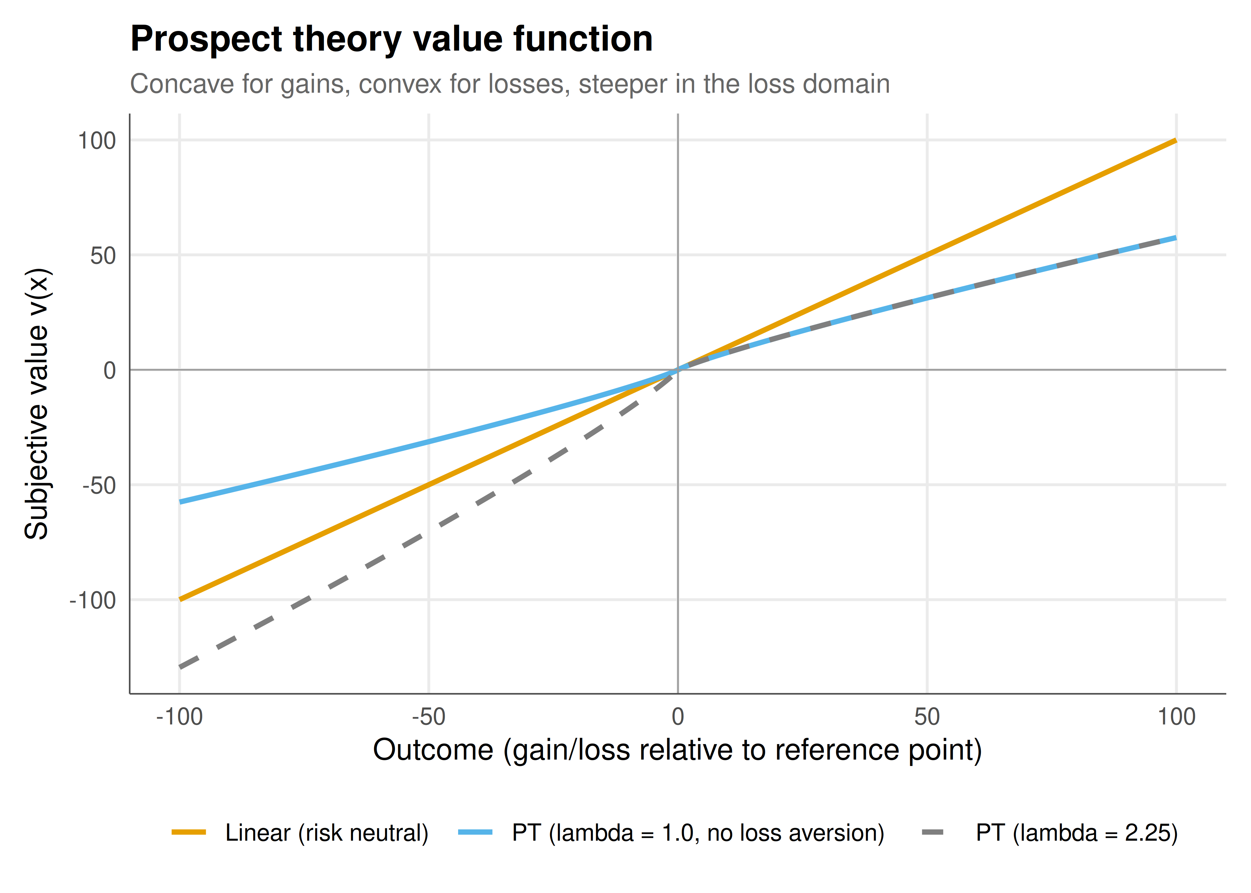
#| fig-cap: "Figure 1. The prospect theory value function compared with a standard utility function. The PT value function (orange) is concave for gains and convex for losses, with a steeper slope in the loss domain reflecting loss aversion (lambda = 2.25). The linear reference (grey dashed) shows risk neutrality. Parameters: alpha = beta = 0.88, lambda = 2.25 (Tversky & Kahneman 1992). Okabe-Ito palette."
#| dev: [png, pdf]
#| fig-width: 7
#| fig-height: 5
#| dpi: 300
x_seq <- seq(-100, 100, by = 0.5)
vf_df <- tibble(
  x = rep(x_seq, 3),
  value = c(pt_value(x_seq, alpha = 0.88, beta = 0.88, lambda = 2.25),
            pt_value(x_seq, alpha = 0.88, beta = 0.88, lambda = 1.0),
            x_seq),
  type = rep(c("PT (lambda = 2.25)", "PT (lambda = 1.0, no loss aversion)", "Linear (risk neutral)"),
             each = length(x_seq))
)

ggplot(vf_df, aes(x = x, y = value, color = type, linetype = type)) +
  geom_line(linewidth = 1) +
  geom_hline(yintercept = 0, color = "grey60", linewidth = 0.3) +
  geom_vline(xintercept = 0, color = "grey60", linewidth = 0.3) +
  scale_color_manual(
    values = c(okabe_ito[1], okabe_ito[2], "grey50"),
    name = NULL
  ) +
  scale_linetype_manual(
    values = c("solid", "solid", "dashed"),
    name = NULL
  ) +
  labs(
    title = "Prospect theory value function",
    subtitle = "Concave for gains, convex for losses, steeper in the loss domain",
    x = "Outcome (gain/loss relative to reference point)",
    y = "Subjective value v(x)"
  ) +
  theme_publication()
```
## Interactive figure
```{r}
#| label: fig-pt-weighting-interactive
p_seq <- seq(0.01, 0.99, by = 0.01)
pw_df <- tibble(
  p = rep(p_seq, 3),
  weighted = c(pt_weight(p_seq, gamma = 0.61),
               pt_weight(p_seq, gamma = 0.69),
               p_seq),
  type = rep(c("Gains (gamma = 0.61)", "Losses (gamma = 0.69)", "Identity (no distortion)"),
             each = length(p_seq))
)

pw_df <- pw_df |>
  mutate(text = paste0("Objective p = ", round(p, 2),
                       "\nWeighted w(p) = ", round(weighted, 3),
                       "\n", type))

p_pw <- ggplot(pw_df, aes(x = p, y = weighted, color = type, text = text)) +
  geom_line(linewidth = 1) +
  scale_color_manual(
    values = c(okabe_ito[1], okabe_ito[3], "grey50"),
    name = NULL
  ) +
  labs(
    title = "Probability weighting functions",
    subtitle = "Overweighting of small probabilities, underweighting of large ones",
    x = "Objective probability p",
    y = "Decision weight w(p)"
  ) +
  theme_publication()

ggplotly(p_pw, tooltip = "text") |>
  config(displaylogo = FALSE,
         modeBarButtonsToRemove = c("select2d", "lasso2d"))
```
## Interpretation
Prospect theory's two departures from expected utility — the S-shaped value function and the inverse-S probability weighting — together generate the **fourfold pattern** of risk attitudes that EU theory cannot accommodate. For gains with moderate-to-high probabilities, the concave value function produces risk aversion (preferring a sure $3000 over an 80% chance at $4000). For gains with small probabilities, overweighting dominates and produces risk seeking (buying lottery tickets). For losses with moderate-to-high probabilities, the convex value function produces risk seeking (gambling to avoid a sure loss). For losses with small probabilities, overweighting again dominates and produces risk aversion (buying insurance against rare catastrophes). The loss aversion parameter $\lambda \approx 2.25$ means that losing $100 feels about as bad as gaining $225 feels good, explaining why people reject symmetric coin-flip gambles that EU theory says they should accept. These predictions have been confirmed in hundreds of experiments and field studies across cultures. Prospect theory's influence extends well beyond academic psychology: it underpins regulatory nudge units (like the UK's Behavioural Insights Team), explains financial anomalies such as the equity premium puzzle and disposition effect, and informs the design of insurance products, tax policy, and marketing strategies. The reference-dependence insight alone has reshaped how economists think about preferences, revealing that context and framing matter as much as final outcomes.
## Extensions & related tutorials
- [The ultimatum game and fairness](../../behavioral-gt/ultimatum-game-fairness/) — behavioural deviations from rationality in strategic settings.
- [Risk dominance and equilibrium selection](../../foundations/risk-dominance/) — how risk attitudes shape equilibrium play.
- [Bayesian games with incomplete information](../../bayesian-methods/bayesian-games-incomplete-information/) — modelling uncertainty about preferences.
- [Nudge design and libertarian paternalism](../nudge-libertarian-paternalism/) — policy applications of prospect theory.
- [Mental accounting and narrow framing](../mental-accounting/) — extensions of reference-dependent preferences.
## References
::: {#refs}
:::