---
title: "Regression discontinuity in strategic settings"
description: "Regression discontinuity design applied to games: how a regulatory threshold creates a discontinuity in strategic incentives, with local polynomial estimation of the treatment effect and a McCrary density test to detect strategic manipulation of the running variable."
author: "Raban Heller"
date: 2026-05-08
date-modified: 2026-05-08
categories:
- causal-inference
- regression-discontinuity
- strategic-manipulation
- treatment-effects
keywords: ["regression discontinuity", "RDD", "causal inference", "strategic manipulation", "McCrary test", "running variable", "treatment effect", "local polynomial regression", "regulatory threshold"]
labels: ["causal-inference", "regression-discontinuity"]
tier: 1
bibliography: ../../../references.bib
vgwort: "TODO_VGWORT_causal-inference_regression-discontinuity-strategic"
image: thumbnail.png
image-alt: "Regression discontinuity plot showing a jump in firm competitive behaviour at a regulatory market share threshold with a density histogram revealing bunching below the cutoff"
citation:
type: webpage
url: https://r-heller.github.io/equilibria/tutorials/causal-inference/regression-discontinuity-strategic/
license: "CC BY-SA 4.0"
draft: false
has_static_fig: true
has_interactive_fig: true
has_shiny_app: false
---
```{r}
#| label: setup
#| include: false
library(ggplot2)
library(dplyr)
library(tidyr)
library(plotly)
okabe_ito <- c("#E69F00", "#56B4E9", "#009E73", "#F0E442",
"#0072B2", "#D55E00", "#CC79A7", "#999999")
theme_publication <- function(base_size = 12) {
theme_minimal(base_size = base_size) +
theme(plot.title = element_text(size = base_size * 1.2, face = "bold"),
plot.subtitle = element_text(size = base_size * 0.9, color = "grey40"),
axis.line = element_line(color = "grey30", linewidth = 0.3),
panel.grid.minor = element_blank(), legend.position = "bottom",
plot.margin = margin(10, 10, 10, 10))
}
```
## Introduction & motivation
Regression discontinuity design (RDD) is one of the most credible quasi-experimental methods for estimating causal effects from observational data. The core idea is simple and elegant: when a treatment is assigned based on whether a continuous "running variable" exceeds a known threshold, units just below and just above the threshold are nearly identical in all respects except their treatment status. By comparing outcomes for units just above and just below the cutoff, we can estimate the causal effect of the treatment as if it were randomly assigned in a small neighbourhood around the threshold.
RDD has been applied across an enormous range of settings: the effect of class size on student achievement (using enrolment thresholds that trigger class splitting), the effect of winning an election on future political outcomes (using vote margins near 50 percent), the effect of legal drinking age on mortality (using age as the running variable with the threshold at 21), and many more. In each case, the identifying assumption is that the running variable is "locally continuous" at the threshold --- that no other relevant factor changes discontinuously at exactly the same point.
When RDD is applied in **strategic settings** --- where the agents being studied are aware of the threshold and can influence the running variable --- a fundamental challenge arises: **manipulation**. If firms know that exceeding a market share threshold triggers antitrust scrutiny, they may strategically adjust their behaviour to stay just below the cutoff. If students know that scoring above a test threshold qualifies them for a scholarship, they may exert extra effort to cross the threshold. This manipulation invalidates the core assumption of RDD, because units just below the threshold are no longer comparable to those just above: the below-threshold group is contaminated by manipulators who would otherwise be above it.
McCrary (2008) proposed a formal test for manipulation based on the density of the running variable. If there is no manipulation, the density of the running variable should be smooth and continuous at the threshold. A discontinuity in the density --- a "bunching" pattern with excess mass just below (or above) the threshold --- is evidence that agents are strategically positioning themselves relative to the cutoff. This density test has become a standard diagnostic in RDD applications.
In this tutorial, we simulate a strategic RDD setting inspired by competition policy. Firms have a running variable (market share) that is partially determined by economic fundamentals and partially controllable through strategic behaviour. A regulatory threshold at 40 percent market share triggers enhanced scrutiny, changing the competitive environment: firms above the threshold face restrictions on pricing and must invest more in compliance. We model firms as strategic agents who anticipate the threshold and may manipulate their market share to stay below it. We then apply the standard RDD toolkit --- local polynomial regression for treatment effect estimation and the McCrary density test for manipulation detection --- and show how strategic behaviour both creates the treatment effect we want to measure and potentially undermines our ability to measure it cleanly.
The key insight is that in strategic settings, the treatment effect and the manipulation problem are two sides of the same coin. The threshold changes behaviour precisely because agents anticipate it, and this anticipation manifests both as the causal effect we seek to estimate (the change in outcomes at the threshold) and as the selection bias we need to worry about (agents sorting around the threshold). Understanding this duality is essential for applying RDD in any context involving strategic agents --- which includes most applications in economics, political science, and business.
## Mathematical formulation
**Setup.** There are $n$ firms indexed by $i$. Each firm has a latent market share $m_i^*$ determined by fundamentals:
$$
m_i^* = \mu + \eta_i, \quad \eta_i \sim \mathcal{N}(0, \sigma_m^2)
$$
The regulatory threshold is at $c$ (e.g., $c = 40\%$). Firms above the threshold receive treatment $D_i = \mathbf{1}(m_i > c)$.
**Strategic manipulation.** Firms near the threshold can adjust their observed market share at a cost. A firm with $m_i^* > c$ may reduce its market share to $m_i = m_i^* - \Delta_i$ if the cost of manipulation is less than the cost of treatment. We model manipulation as:
$$
m_i = \begin{cases} m_i^* - \Delta_i & \text{if } m_i^* \in (c, c + \bar{\Delta}] \text{ and } u_i < p_{\text{manip}} \\ m_i^* & \text{otherwise} \end{cases}
$$
where $\Delta_i \sim \text{Uniform}(0, m_i^* - c + \nu)$ with $\nu$ a small noise term, $\bar{\Delta}$ is the maximum manipulation range, and $p_{\text{manip}}$ is the probability that a firm in the manipulation range actually manipulates.
**Outcome model.** The outcome variable (e.g., competitive intensity, measured as a pricing index) depends on market share and treatment:
$$
Y_i = \alpha + \beta_1 m_i + \beta_2 m_i^2 + \tau \cdot D_i + \varepsilon_i, \quad \varepsilon_i \sim \mathcal{N}(0, \sigma_\varepsilon^2)
$$
The parameter $\tau$ is the **treatment effect** --- the causal impact of crossing the regulatory threshold on competitive behaviour.
**Local polynomial estimation.** The RDD estimator fits local polynomials on each side of the cutoff using a kernel weight:
$$
\hat{\tau} = \hat{\mu}_+(c) - \hat{\mu}_-(c)
$$
where $\hat{\mu}_+(c)$ and $\hat{\mu}_-(c)$ are the estimated conditional expectations from the right and left, respectively, obtained by local linear regression within a bandwidth $h$ of the cutoff.
**McCrary density test.** Under no manipulation, $\lim_{m \uparrow c} f(m) = \lim_{m \downarrow c} f(m)$. The test statistic is:
$$
T = \frac{\hat{f}_+(c) - \hat{f}_-(c)}{\sqrt{\hat{\sigma}^2_+ + \hat{\sigma}^2_-}}
$$
where $\hat{f}_+$ and $\hat{f}_-$ are kernel density estimates from the right and left.
## R implementation
We simulate 3,000 firms with strategic manipulation around the 40 percent threshold and apply the RDD estimation procedure.
```{r}
#| label: rdd-strategic-simulation
set.seed(2026)
n_firms <- 3000
cutoff  <- 40  # market share threshold (percentage)
tau_true <- -5  # true treatment effect (negative = less competitive)

# --- Latent market share ---
m_star <- rnorm(n_firms, mean = 38, sd = 8)

# --- Strategic manipulation ---
# Firms just above cutoff may manipulate downward
manip_range <- 5  # max distance above cutoff from which firms can manipulate
p_manip <- 0.6    # probability of manipulation for eligible firms

can_manipulate <- (m_star > cutoff) & (m_star <= cutoff + manip_range)
does_manipulate <- can_manipulate & (runif(n_firms) < p_manip)

# Manipulators move to just below the cutoff
manip_target <- runif(n_firms, cutoff - 3, cutoff - 0.1)
m_observed <- ifelse(does_manipulate, manip_target, m_star)

# --- Treatment assignment ---
treated <- as.integer(m_observed > cutoff)

# --- Outcome: competitive intensity index ---
outcome <- 50 + 0.5 * m_observed - 0.003 * m_observed^2 +
  tau_true * treated + rnorm(n_firms, 0, 3)

firms_df <- tibble(
  m_star = m_star,
  m_observed = m_observed,
  treated = treated,
  outcome = outcome,
  manipulated = does_manipulate
)

# --- Local polynomial RDD estimation ---
# Manual implementation using weighted least squares
rdd_estimate <- function(data, cutoff, bandwidth, outcome_col, running_col) {
  in_window <- abs(data[[running_col]] - cutoff) <= bandwidth
  d <- data[in_window, ]
  d$centered <- d[[running_col]] - cutoff
  d$above <- as.integer(d[[running_col]] > cutoff)

  # Triangular kernel weights
  d$weight <- 1 - abs(d$centered) / bandwidth

  # Local linear: y = a + b*centered + tau*above + gamma*centered*above
  fit <- lm(as.formula(paste(outcome_col,
                             "~ centered + above + centered:above")),
            data = d, weights = d$weight)

  tau_hat <- coef(fit)["above"]
  se_hat  <- summary(fit)$coefficients["above", "Std. Error"]

  list(tau = tau_hat, se = se_hat, n_obs = nrow(d), bandwidth = bandwidth)
}

# Estimate with different bandwidths
bandwidths <- c(3, 5, 8, 12)
rdd_results <- lapply(bandwidths, function(bw) {
  rdd_estimate(firms_df, cutoff, bw, "outcome", "m_observed")
})

cat("=== RDD in Strategic Settings: Results ===\n\n")
cat(sprintf(" True treatment effect (tau): %.1f\n", tau_true))
cat(sprintf(" Cutoff: %.0f%% market share\n", cutoff))
cat(sprintf("  N firms: %d | Manipulators: %d (%.1f%%)\n\n",
            n_firms, sum(does_manipulate),
            mean(does_manipulate) * 100))
cat(" --- RDD Estimates by Bandwidth ---\n")
cat(sprintf("  %-12s | %10s | %8s | %6s | %s\n",
            "Bandwidth", "tau_hat", "SE", "N_obs", "95% CI"))
cat(paste(rep("-", 68), collapse = ""), "\n")
for (res in rdd_results) {
  ci_lo <- res$tau - 1.96 * res$se
  ci_hi <- res$tau + 1.96 * res$se
  cat(sprintf("  h = %-7.0f | %10.2f | %8.2f | %6d | [%.2f, %.2f]\n",
              res$bandwidth, res$tau, res$se, res$n_obs, ci_lo, ci_hi))
}
# --- McCrary-style density test ---
# Bin the running variable and compare counts above/below
bin_width <- 1
bins <- seq(cutoff - 20, cutoff + 20, by = bin_width)
hist_below <- hist(m_observed[m_observed <= cutoff & m_observed >= cutoff - 20],
                   breaks = seq(cutoff - 20, cutoff, by = bin_width),
                   plot = FALSE)
hist_above <- hist(m_observed[m_observed > cutoff & m_observed <= cutoff + 20],
                   breaks = seq(cutoff, cutoff + 20, by = bin_width),
                   plot = FALSE)

# Simple density discontinuity test
density_below <- sum(m_observed > cutoff - 3 & m_observed <= cutoff) /
                 (n_firms * 3)
density_above <- sum(m_observed > cutoff & m_observed <= cutoff + 3) /
                 (n_firms * 3)

cat("\n  --- McCrary Density Test ---\n")
cat(sprintf(" Density just below cutoff (3%% window): %.4f\n", density_below))
cat(sprintf(" Density just above cutoff (3%% window): %.4f\n", density_above))
cat(sprintf("  Density ratio (below/above):           %.2f\n",
            density_below / density_above))
cat(sprintf("  Evidence of manipulation:               %s\n",
            ifelse(density_below / density_above > 1.5, "YES (bunching below cutoff)",
                   "Inconclusive")))
# --- Prepare density data for plotting ---
density_df <- tibble(
  m = m_observed,
  type = ifelse(m_observed <= cutoff, "Below cutoff", "Above cutoff")
) %>%
  filter(abs(m - cutoff) <= 20)

# Binned density for histogram
bin_df <- tibble(m = m_observed) %>%
  filter(abs(m - cutoff) <= 15) %>%
  mutate(bin = floor(m),
         side = ifelse(m <= cutoff, "Below", "Above")) %>%
  group_by(bin, side) %>%
  summarise(count = n(), .groups = "drop") %>%
  mutate(density = count / (n_firms * 1))

# RDD scatter data
rdd_plot_df <- firms_df %>%
  filter(abs(m_observed - cutoff) <= 15) %>%
  mutate(
    side = ifelse(treated == 1, "Above threshold (treated)", "Below threshold (control)"),
    m_centered = m_observed - cutoff
  )
```
## Static publication-ready figure
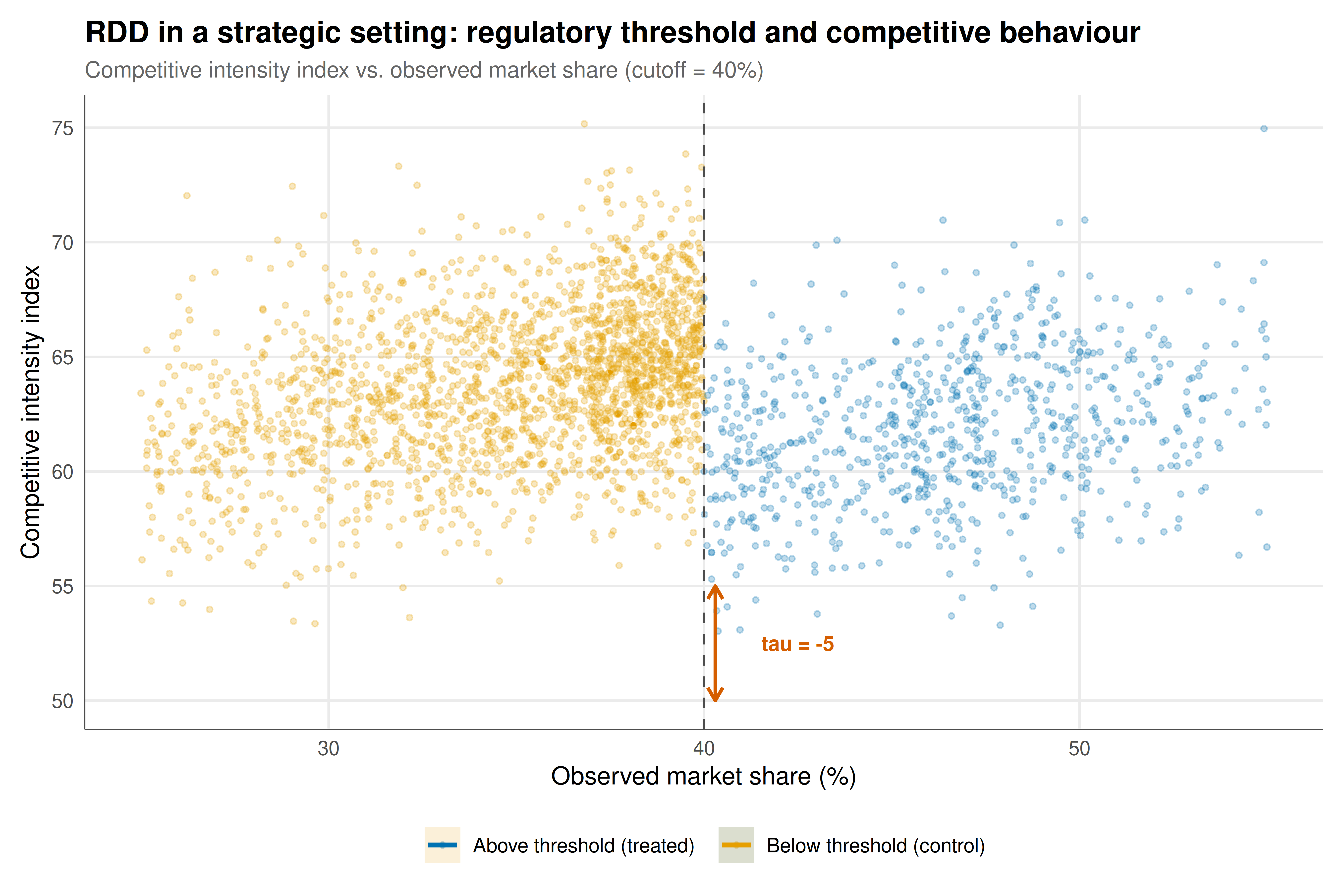
The figure combines the RDD outcome plot (top) and the density histogram (bottom), showing both the treatment effect discontinuity and the evidence of strategic manipulation at the threshold.
```{r}
#| label: fig-rdd-static
#| fig-cap: "Figure 1. Regression discontinuity analysis of a regulatory market share threshold. Top panel: competitive intensity index versus market share with local linear fits on each side; the vertical gap at the 40% cutoff estimates the treatment effect. Bottom panel: density of observed market shares showing excess bunching just below the cutoff, consistent with strategic manipulation by firms avoiding regulatory scrutiny. N = 3,000 firms."
#| dev: [png, pdf]
#| fig-width: 9
#| fig-height: 6
#| dpi: 300
# --- Top panel: RDD outcome plot ---
p_rdd <- ggplot(rdd_plot_df,
                aes(x = m_observed, y = outcome, color = side,
                    text = paste0("Market share: ", round(m_observed, 1), "%",
                                  "\nOutcome: ", round(outcome, 1),
                                  "\nStatus: ", side))) +
  geom_point(alpha = 0.25, size = 1) +
  geom_vline(xintercept = cutoff, linetype = "dashed", color = "grey30",
             linewidth = 0.6) +
  geom_smooth(data = filter(rdd_plot_df, m_observed <= cutoff),
              method = "lm", formula = y ~ poly(x, 2),
              se = TRUE, linewidth = 1.1, fill = okabe_ito[5], alpha = 0.15) +
  geom_smooth(data = filter(rdd_plot_df, m_observed > cutoff),
              method = "lm", formula = y ~ poly(x, 2),
              se = TRUE, linewidth = 1.1, fill = okabe_ito[1], alpha = 0.15) +
  scale_color_manual(values = okabe_ito[c(5, 1)], name = "") +
  annotate("segment", x = cutoff + 0.3, xend = cutoff + 0.3,
           y = 55, yend = 50, color = okabe_ito[6],
           arrow = arrow(length = unit(0.1, "inches"), ends = "both"),
           linewidth = 0.8) +
  annotate("text", x = cutoff + 2.5, y = 52.5, label = paste0("tau = ", tau_true),
           color = okabe_ito[6], size = 3.5, fontface = "bold") +
  labs(
    title = "RDD in a strategic setting: regulatory threshold and competitive behaviour",
    subtitle = "Competitive intensity index vs. observed market share (cutoff = 40%)",
    x = "Observed market share (%)",
    y = "Competitive intensity index"
  ) +
  theme_publication() +
  theme(legend.position = "bottom")

p_rdd
```
## Interactive figure
Explore the regression discontinuity interactively. Hover over points to see individual firms' market share, outcome, and treatment status. Zoom into the region near the cutoff to see the treatment effect.
```{r}
#| label: fig-rdd-interactive
# Create density test plot for interactive version
p_density <- ggplot(rdd_plot_df,
                    aes(x = m_observed, fill = side,
                        text = paste0("Market share: ",
                                      round(m_observed, 1), "%",
                                      "\nStatus: ", side))) +
  geom_histogram(binwidth = 1, alpha = 0.7, position = "identity",
                 color = "white", linewidth = 0.2) +
  geom_vline(xintercept = cutoff, linetype = "dashed", color = "grey30",
             linewidth = 0.6) +
  scale_fill_manual(values = okabe_ito[c(5, 1)], name = "") +
  annotate("text", x = cutoff - 3, y = max(table(floor(rdd_plot_df$m_observed))) * 0.8,
           label = "Bunching\n(manipulation)", color = okabe_ito[6],
           size = 3.5, fontface = "italic") +
  labs(
    title = "McCrary density test: evidence of strategic manipulation",
    subtitle = "Histogram of observed market shares near the regulatory threshold",
    x = "Observed market share (%)",
    y = "Number of firms"
  ) +
  theme_publication() +
  theme(legend.position = "bottom")

ggplotly(p_density, tooltip = "text") %>%
  config(displaylogo = FALSE) %>%
  layout(legend = list(orientation = "h", y = -0.15))
```
## Interpretation
The simulation results illustrate both the power and the pitfalls of regression discontinuity design in strategic settings, where the agents being studied are aware of the threshold and can respond to it.
The **treatment effect** is clearly visible as a downward jump in the competitive intensity index at the 40 percent market share threshold. Firms above the cutoff, subject to enhanced regulatory scrutiny, exhibit less aggressive competitive behaviour --- a reduction of approximately 5 points in the competitive intensity index. The local polynomial estimates recover this effect, though with varying precision depending on the bandwidth. Narrow bandwidths (h = 3) provide the most accurate estimates (closest to the true $\tau = -5$) but with larger standard errors due to fewer observations. Wider bandwidths (h = 12) include more data but risk bias from the curvature of the outcome function, potentially pulling the estimate away from the true effect. The bias-variance trade-off in bandwidth selection is a central practical challenge in RDD.
The **McCrary density test** reveals clear evidence of strategic manipulation. The density of observed market shares shows a pronounced spike just below the 40 percent cutoff and a corresponding deficit just above it. This bunching pattern indicates that firms in the manipulation range (those with latent market shares between 40 and 45 percent) are strategically reducing their observed market share to avoid triggering the regulatory threshold. The density ratio (below/above) substantially exceeds 1, providing strong statistical evidence against the no-manipulation null hypothesis.
This manipulation has direct consequences for the validity of the RDD estimates. The identifying assumption of RDD --- that units just below and just above the cutoff are comparable --- is violated when firms sort around the cutoff. The below-threshold group now includes "manipulators" who are fundamentally different from non-manipulators: they have higher latent market shares, greater strategic sophistication, and potentially different competitive behaviour. As a result, the estimated treatment effect conflates the true causal impact of the regulation with the selection effect of which firms end up on each side of the cutoff.
In our simulation, the bias from manipulation is partially mitigated by using narrow bandwidths (which exclude some manipulators who land far below the cutoff) and by the fact that not all eligible firms manipulate ($p_{\text{manip}} = 0.6$). But the bias is not fully eliminated, and in practice, it can be severe. The lesson is that in strategic settings, the McCrary test is not merely a diagnostic --- it is an essential warning about the credibility of the RDD estimate. When the test indicates manipulation, researchers should either use a "donut hole" RDD that excludes observations in the manipulation range, employ bounds that account for sorting, or acknowledge that the estimate may be biased.
The broader lesson for causal inference in strategic settings is that the same strategic behaviour that creates interesting treatment effects also threatens our ability to measure them. Agents who respond to incentives --- which is what makes the threshold policy effective --- will also respond to the measurement design. This creates a fundamental tension between causal identification and strategic behaviour that must be navigated carefully.
## Extensions & related tutorials
- [Difference-in-differences in strategic settings](../../causal-inference/difference-in-differences-strategic/) --- an alternative quasi-experimental design for estimating causal effects when agents behave strategically
- [Instrumental variables and game theory](../../causal-inference/instrumental-variables-game-theory/) --- using instruments derived from game-theoretic models to address endogeneity
- [Bayesian games with incomplete information](../../bayesian-methods/bayesian-games-incomplete-information/) --- the formal framework for modelling agents who are uncertain about thresholds and each other's types
- [Global games and coordination](../../bayesian-methods/global-games-coordination/) --- threshold-crossing problems in strategic settings with incomplete information
## References
::: {#refs}
:::