---
title: "Blockchain consensus as a game"
description: "Model Proof-of-Work mining as a strategic game among heterogeneous miners, analyse Nash equilibrium hash rate allocation, simulate 51% attack incentives as a coordination game, and explore mining pool formation through coalition game theory."
author: "Raban Heller"
date: 2026-05-08
date-modified: 2026-05-08
categories:
- cryptography-and-gt
- blockchain
- mining-game
- coalition-formation
keywords: ["blockchain", "Proof-of-Work", "mining game", "Nash equilibrium", "51% attack", "mining pool", "hash rate", "coalition game", "consensus mechanism", "game theory"]
labels: ["cryptography-and-gt", "mechanism-design"]
tier: 1
bibliography: ../../../references.bib
vgwort: "TODO_VGWORT_cryptography-and-gt_blockchain-consensus-game"
image: thumbnail.png
image-alt: "Chart showing Nash equilibrium hash rate allocation among heterogeneous miners and profitability thresholds in a Proof-of-Work mining game"
citation:
type: webpage
url: https://r-heller.github.io/equilibria/tutorials/cryptography-and-gt/blockchain-consensus-game/
license: "CC BY-SA 4.0"
draft: false
has_static_fig: true
has_interactive_fig: true
has_shiny_app: false
---
```{r}
#| label: setup
#| include: false
library(ggplot2)
library(dplyr)
library(tidyr)
library(plotly)
okabe_ito <- c("#E69F00", "#56B4E9", "#009E73", "#F0E442",
"#0072B2", "#D55E00", "#CC79A7", "#999999")
theme_publication <- function(base_size = 12) {
theme_minimal(base_size = base_size) +
theme(plot.title = element_text(size = base_size * 1.2, face = "bold"),
plot.subtitle = element_text(size = base_size * 0.9, color = "grey40"),
axis.line = element_line(color = "grey30", linewidth = 0.3),
panel.grid.minor = element_blank(), legend.position = "bottom",
plot.margin = margin(10, 10, 10, 10))
}
```
## Introduction & motivation
Blockchain consensus mechanisms are, at their core, game-theoretic protocols. In a Proof-of-Work (PoW) system like Bitcoin, miners compete to solve cryptographic puzzles by investing computational resources (hash power). The miner who finds a valid block first receives a block reward (newly minted cryptocurrency plus transaction fees). Each miner's probability of winning is proportional to their share of total network hash power. This creates a strategic environment where each miner must decide how much hash power to deploy, balancing the cost of computation against the expected block reward.
The game-theoretic structure of PoW mining has several layers. At the most basic level, mining is a **contest game**: players invest costly effort (hash power) to compete for a fixed prize (block reward), and the probability of winning is proportional to relative effort. This is a well-studied class of games with known Nash equilibrium properties. In equilibrium, miners invest up to the point where their marginal cost of additional hash power equals the marginal increase in expected reward. Miners with lower costs per hash (more efficient hardware, cheaper electricity) invest more and earn higher profits; miners with sufficiently high costs exit the market.
At a deeper level, the security of the blockchain itself depends on the game-theoretic incentives being aligned. The infamous **51% attack** illustrates this: if a single miner (or coordinated coalition of miners) controls more than half the network's hash power, they can manipulate the blockchain by double-spending transactions or censoring blocks. The attack is a **coordination game** among potential attackers: the attack is only profitable if enough miners join the coalition to exceed the 51% threshold, creating a strategic complementarity. In a healthy network, the Nash equilibrium of this coordination game is "no attack" --- honest mining is more profitable than attacking. But when the block reward declines (as in Bitcoin's halving schedule) or transaction fees are insufficient, the incentive structure can shift, making the attack equilibrium viable.
A third game-theoretic dimension is **mining pool formation**. Individual miners face high variance in rewards (a solo miner might wait months between finding a block), so they form pools that share rewards proportionally. Pool formation is a **coalition game**: miners must decide which pool to join, and the pool must decide how to divide rewards among members. The Shapley value and the core of this cooperative game determine fair and stable reward divisions.
In this tutorial, we model all three layers. We compute the Nash equilibrium of the mining contest game with heterogeneous miners, analyse the 51% attack as a coordination game, simulate mining dynamics with stochastic block discovery, and explore pool formation incentives. The analysis demonstrates how game theory provides both a descriptive model of actual blockchain behaviour and a normative framework for designing better consensus mechanisms.
## Mathematical formulation
**Mining contest game.** There are $N$ miners, each choosing hash rate $h_i \geq 0$. The cost of mining at rate $h_i$ is $c_i \cdot h_i$ (linear cost, where $c_i$ is miner $i$'s cost per hash). The block reward is $R$. Miner $i$'s expected payoff per block is:
$$
\pi_i(h_i, h_{-i}) = \frac{h_i}{\sum_{j=1}^N h_j} \cdot R - c_i \cdot h_i
$$
**Nash equilibrium.** Taking the first-order condition $\partial \pi_i / \partial h_i = 0$:
$$
\frac{\sum_{j \neq i} h_j}{\left(\sum_{j=1}^N h_j\right)^2} \cdot R = c_i
$$
Let $H = \sum_j h_j$ be total hash rate and $H_{-i} = H - h_i$. Then:
$$
h_i^* = H^* - \frac{c_i \cdot (H^*)^2}{R}
$$
For $N$ symmetric miners with cost $c$, the equilibrium hash rate is:
$$
h_i^* = \frac{(N-1)R}{N^2 c}, \quad H^* = \frac{(N-1)R}{Nc}
$$
**51% attack as coordination game.** Let $A$ be the set of attacking miners with combined hash rate $H_A$. The attack succeeds if $H_A / H > 0.5$. The payoff from a successful attack is $V$ (value of double-spend), shared proportionally among attackers. The cost is the opportunity cost of not mining honestly during the attack plus the risk of the cryptocurrency losing value. This creates a coordination game where the attack is an equilibrium only if:
$$
\frac{h_i}{H_A} \cdot V - c_i \cdot h_i \cdot \Delta t > \frac{h_i}{H} \cdot R \cdot \Delta t
$$
**Pool formation (cooperative game).** Define the characteristic function $v(S)$ as the expected payoff of coalition $S$ mining as a pool:
$$
v(S) = \frac{\sum_{i \in S} h_i}{H} \cdot R - \sum_{i \in S} c_i h_i
$$
The **Shapley value** for miner $i$ gives a fair allocation based on marginal contributions across all possible coalition orderings.
## R implementation
We compute the Nash equilibrium for heterogeneous miners, simulate the mining game dynamics, analyse 51% attack incentives, and compute pool formation values.
```{r}
#| label: blockchain-computation
# --- Mining Contest Game: Nash Equilibrium ---
compute_mining_ne <- function(costs, R = 6.25) {
  N <- length(costs)
  # Solve for H* numerically
  # FOC: for active miner i, h_i = H - c_i * H^2 / R
  # Sum: H = N*H - H^2/R * sum(c_i)  =>  H*(N-1) = H^2/R * sum(c_active)
  # H* = (N-1)*R / sum(c_active) for active miners

  # Iterative: start with all miners active, remove unprofitable ones
  active <- rep(TRUE, N)
  for (iter in 1:N) {
    n_active <- sum(active)
    if (n_active == 0) break
    c_active <- costs[active]
    H_star <- (n_active - 1) * R / sum(c_active)

    h_star <- rep(0, N)
    h_star[active] <- H_star - costs[active] * H_star^2 / R

    # Check for negative hash rates (miners should exit)
    new_active <- h_star > 0
    if (all(new_active == active)) break
    active <- new_active
  }

  h_star <- pmax(h_star, 0)
  H_total <- sum(h_star)
  profits <- ifelse(H_total > 0, h_star / H_total * R - costs * h_star, 0)

  tibble(
    miner = paste0("M", 1:N),
    cost = costs,
    hash_rate = h_star,
    share = ifelse(H_total > 0, h_star / H_total, 0),
    revenue = ifelse(H_total > 0, h_star / H_total * R, 0),
    cost_total = costs * h_star,
    profit = profits,
    active = h_star > 0
  )
}

# Heterogeneous miners: 8 miners with different costs
miner_costs <- c(0.02, 0.025, 0.03, 0.035, 0.04, 0.05, 0.06, 0.08)
R <- 6.25  # Block reward in BTC (post-2024 halving)

ne_result <- compute_mining_ne(miner_costs, R)

cat("=== Mining Nash Equilibrium (R = 6.25 BTC) ===\n\n")
ne_result %>%
  mutate(across(c(hash_rate, share, revenue, cost_total, profit),
                ~ round(., 4))) %>%
  print(n = 10)
cat(sprintf("\nTotal hash rate: %.4f\n", sum(ne_result$hash_rate)))
cat(sprintf("Active miners: %d / %d\n", sum(ne_result$active), nrow(ne_result)))
# --- 51% Attack Analysis ---
# Model: attacker coalition needs > 50% of hash rate
# Cost: opportunity cost of honest mining during attack duration
attack_analysis <- function(ne, attack_value = 100, attack_duration = 6) {
  H_total <- sum(ne$hash_rate)
  n <- nrow(ne)

  # For each possible coalition (sorted by cost efficiency)
  ne_sorted <- ne %>% arrange(cost)
  cum_share <- cumsum(ne_sorted$hash_rate) / H_total

  # Find minimum coalition for 51%
  min_coalition_size <- which(cum_share > 0.5)[1]

  # Attack payoff vs honest mining payoff for the coalition
  coalition_members <- 1:min_coalition_size
  coalition_hash <- sum(ne_sorted$hash_rate[coalition_members])
  coalition_share <- coalition_hash / H_total

  # Honest payoff for coalition members over attack_duration blocks
  honest_payoff <- sum(ne_sorted$profit[coalition_members]) * attack_duration

  # Attack payoff: double-spend value minus mining costs during attack
  attack_cost <- sum(ne_sorted$cost[coalition_members] *
                       ne_sorted$hash_rate[coalition_members]) * attack_duration
  attack_payoff <- attack_value - attack_cost

  tibble(
    min_coalition_size = min_coalition_size,
    coalition_share = coalition_share,
    honest_payoff = honest_payoff,
    attack_payoff = attack_payoff,
    attack_profitable = attack_payoff > honest_payoff
  )
}

attack_values <- seq(10, 500, by = 10)
attack_results <- tibble(
  attack_value = attack_values,
  profitable = logical(length(attack_values)),
  net_gain = numeric(length(attack_values))
)

for (i in seq_along(attack_values)) {
  res <- attack_analysis(ne_result, attack_value = attack_values[i])
  attack_results$profitable[i] <- res$attack_profitable
  attack_results$net_gain[i] <- res$attack_payoff - res$honest_payoff
}

threshold_value <- attack_results$attack_value[which(attack_results$profitable)[1]]
cat(sprintf("\n=== 51%% Attack Analysis ===\n"))
cat(sprintf("Minimum double-spend value for profitable attack: %.0f BTC\n",
            ifelse(is.na(threshold_value), Inf, threshold_value)))
# --- Mining Dynamics Simulation ---
set.seed(42)
simulate_mining <- function(n_miners = 5, n_blocks = 200, R = 6.25,
                            costs = NULL) {
  if (is.null(costs)) costs <- seq(0.02, 0.05, length.out = n_miners)
  # Start with equal hash rates
  hash_rates <- rep(R / (2 * max(costs) * n_miners), n_miners)

  history <- matrix(0, n_blocks, n_miners + 1)
  colnames(history) <- c(paste0("M", 1:n_miners), "winner")

  for (b in 1:n_blocks) {
    total_hash <- sum(hash_rates)
    win_probs <- hash_rates / total_hash

    # Determine block winner
    winner <- sample(1:n_miners, 1, prob = win_probs)
    history[b, 1:n_miners] <- hash_rates
    history[b, n_miners + 1] <- winner

    # Miners adjust: gradient step toward best response
    for (i in 1:n_miners) {
      H_others <- total_hash - hash_rates[i]
      # Optimal: h_i = sqrt(R * H_others / c_i) - H_others (simplified)
      optimal <- max(0, sqrt(R * H_others / costs[i]) - H_others)
      # Partial adjustment
      hash_rates[i] <- 0.9 * hash_rates[i] + 0.1 * optimal
    }
  }

  list(
    history = as.data.frame(history),
    costs = costs
  )
}

sim <- simulate_mining(n_miners = 5, n_blocks = 300,
                       costs = c(0.02, 0.025, 0.03, 0.04, 0.06))

hash_history <- sim$history[, 1:5] %>%
  mutate(block = 1:n()) %>%
  pivot_longer(cols = -block, names_to = "miner", values_to = "hash_rate")

cat("\n=== Mining Dynamics Simulation ===\n")
cat("Final hash rates:\n")
final_hash <- sim$history[300, 1:5]
names(final_hash) <- paste0("M", 1:5)
print(round(unlist(final_hash), 4))
# --- Pool Formation: Shapley Value ---
compute_shapley <- function(ne, R = 6.25) {
  n <- sum(ne$active)
  active_miners <- ne %>% filter(active)
  h <- active_miners$hash_rate
  c_vec <- active_miners$cost
  H <- sum(h)

  # Characteristic function: v(S) = revenue(S) - cost(S)
  char_fn <- function(S) {
    if (length(S) == 0) return(0)
    h_S <- sum(h[S])
    rev <- h_S / H * R
    cost <- sum(c_vec[S] * h[S])
    rev - cost
  }

  # Compute Shapley value by sampling permutations
  n_perms <- min(factorial(n), 5000)
  shapley <- rep(0, n)

  set.seed(42)
  for (perm_idx in 1:n_perms) {
    perm <- sample(1:n)
    for (pos in 1:n) {
      i <- perm[pos]
      S_before <- if (pos > 1) perm[1:(pos-1)] else integer(0)
      marginal <- char_fn(c(S_before, i)) - char_fn(S_before)
      shapley[i] <- shapley[i] + marginal
    }
  }
  shapley <- shapley / n_perms

  active_miners %>%
    mutate(shapley_value = shapley,
           shapley_share = shapley / sum(shapley))
}

shapley_result <- compute_shapley(ne_result)

cat("\n=== Shapley Values for Mining Pool ===\n")
shapley_result %>%
  select(miner, cost, hash_rate, profit, shapley_value, shapley_share) %>%
  mutate(across(c(hash_rate, profit, shapley_value, shapley_share),
                ~ round(., 4))) %>%
  print(n = 10)
```
## Static publication-ready figure
The figure presents three panels: Nash equilibrium hash rate allocation, attack profitability analysis, and mining dynamics convergence.
```{r}
#| label: fig-blockchain-static
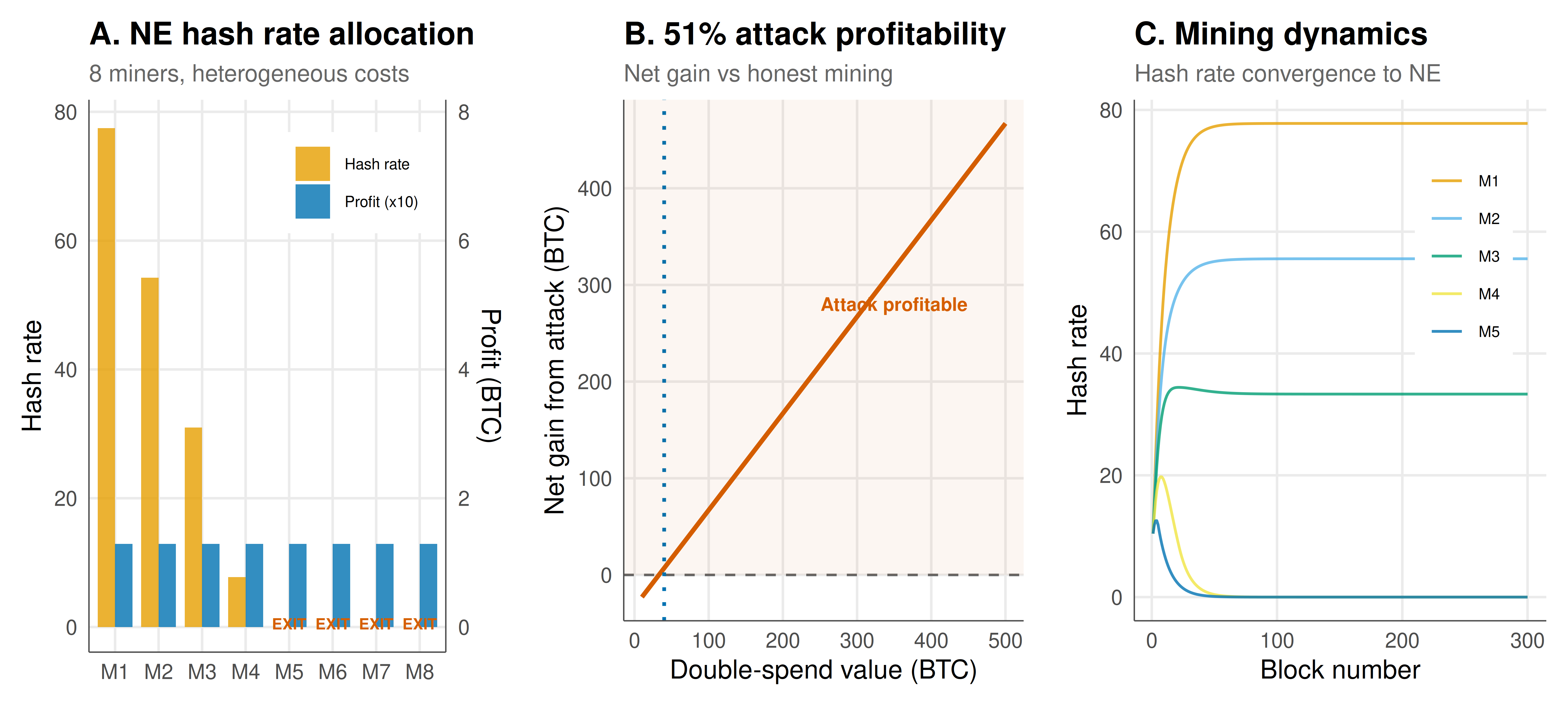
#| fig-cap: "Figure 1. Left: Nash equilibrium hash rate and profit for 8 heterogeneous miners. Low-cost miners (M1-M2) invest more and earn higher profits; high-cost miners (M7-M8) exit the market. Centre: Net gain from a 51% attack as a function of double-spend value, showing the threshold above which attacking becomes profitable. Right: Mining dynamics simulation showing hash rate convergence over 300 blocks for 5 miners with different costs."
#| dev: [png, pdf]
#| fig-width: 10
#| fig-height: 4.5
#| dpi: 300
# Panel A: NE hash rates and profits
ne_plot <- ne_result %>%
  select(miner, hash_rate, profit) %>%
  pivot_longer(cols = c(hash_rate, profit), names_to = "metric", values_to = "value")

p_ne <- ggplot(ne_result, aes(x = miner)) +
  geom_col(aes(y = hash_rate, fill = "Hash rate"), alpha = 0.8, width = 0.4,
           position = position_nudge(x = -0.2)) +
  geom_col(aes(y = profit * 10, fill = "Profit (x10)"), alpha = 0.8, width = 0.4,
           position = position_nudge(x = 0.2)) +
  geom_text(aes(y = hash_rate + 0.5, label = ifelse(active, "", "EXIT")),
            size = 2.5, colour = okabe_ito[6], fontface = "bold") +
  scale_fill_manual(values = okabe_ito[c(1, 5)]) +
  scale_y_continuous(
    name = "Hash rate",
    sec.axis = sec_axis(~ . / 10, name = "Profit (BTC)")
  ) +
  labs(
    title = "A. NE hash rate allocation",
    subtitle = "8 miners, heterogeneous costs",
    x = NULL, fill = NULL
  ) +
  theme_publication() +
  theme(legend.position = c(0.75, 0.85),
        legend.background = element_rect(fill = "white", colour = NA),
        legend.text = element_text(size = 7))

# Panel B: Attack profitability
p_attack <- ggplot(attack_results, aes(x = attack_value, y = net_gain)) +
  geom_line(colour = okabe_ito[6], linewidth = 1) +
  geom_hline(yintercept = 0, linetype = "dashed", colour = "grey40") +
  geom_vline(xintercept = ifelse(is.na(threshold_value), 500, threshold_value),
             linetype = "dotted", colour = okabe_ito[5], linewidth = 0.8) +
  annotate("rect", xmin = -Inf, xmax = Inf, ymin = 0, ymax = Inf,
           fill = okabe_ito[6], alpha = 0.05) +
  annotate("text", x = 350, y = max(attack_results$net_gain) * 0.6,
           label = "Attack profitable", colour = okabe_ito[6],
           size = 3, fontface = "bold") +
  labs(
    title = "B. 51% attack profitability",
    subtitle = "Net gain vs honest mining",
    x = "Double-spend value (BTC)",
    y = "Net gain from attack (BTC)"
  ) +
  theme_publication()

# Panel C: Mining dynamics
p_dynamics <- ggplot(hash_history, aes(x = block, y = hash_rate, colour = miner)) +
  geom_line(linewidth = 0.6, alpha = 0.8) +
  scale_colour_manual(values = okabe_ito[1:5]) +
  labs(
    title = "C. Mining dynamics",
    subtitle = "Hash rate convergence to NE",
    x = "Block number", y = "Hash rate",
    colour = NULL
  ) +
  theme_publication() +
  theme(legend.position = c(0.8, 0.7),
        legend.background = element_rect(fill = "white", colour = NA),
        legend.text = element_text(size = 7))

gridExtra::grid.arrange(p_ne, p_attack, p_dynamics, ncol = 3)
```
## Interactive figure
Explore the mining Nash equilibrium interactively. Hover over each miner's bar to see their cost, hash rate, share, revenue, and profit at equilibrium.
```{r}
#| label: fig-blockchain-interactive
p_int <- ggplot(ne_result,
       aes(x = miner, y = hash_rate, fill = active,
           text = paste0("Miner: ", miner,
                         "\nCost/hash: ", cost,
                         "\nHash rate: ", round(hash_rate, 4),
                         "\nShare: ", round(share * 100, 1), "%",
                         "\nRevenue: ", round(revenue, 4), " BTC",
                         "\nCost: ", round(cost_total, 4), " BTC",
                         "\nProfit: ", round(profit, 4), " BTC",
                         "\nActive: ", active))) +
  geom_col(alpha = 0.8) +
  scale_fill_manual(values = okabe_ito[c(8, 3)],
                    labels = c("Exited", "Active")) +
  labs(
    title = "Mining Nash equilibrium: hash rate allocation by miner",
    x = NULL, y = "Hash rate (equilibrium)",
    fill = "Status"
  ) +
  theme_publication()

ggplotly(p_int, tooltip = "text") %>%
  config(displaylogo = FALSE) %>%
  layout(legend = list(orientation = "h", y = -0.2))
```
## Interpretation
The game-theoretic analysis of blockchain mining reveals several fundamental insights about how decentralised consensus mechanisms work --- and how they can fail.
**Entry and exit in the mining game.** The Nash equilibrium computation shows that not all miners are active in equilibrium. Miners with costs exceeding a threshold exit the market because the expected reward does not cover their costs. This mirrors the real-world observation that less efficient mining operations shut down during bear markets or after block reward halvings. The equilibrium is self-regulating: as high-cost miners exit, the remaining miners earn higher shares of the block reward, and total hash rate adjusts to a level where the marginal miner is indifferent between mining and not mining.
**Cost heterogeneity drives concentration.** Low-cost miners (with access to cheap electricity, efficient hardware, or economies of scale) invest more hash power and earn disproportionately high profits. This is a direct consequence of the contest structure: in equilibrium, each miner's investment is proportional to their cost advantage. The resulting hash rate distribution is skewed, with a small number of efficient miners controlling a large share of total hash power. This concentration has implications for decentralisation --- the foundational premise of blockchain technology --- and for the feasibility of 51% attacks.
**The 51% attack threshold depends on the economic environment.** Our analysis shows that the profitability of a 51% attack is a function of the double-spend value relative to the honest mining profits of the attacking coalition. When block rewards are high and the potential double-spend value is low, honest mining is the dominant strategy. But as block rewards decline (due to halving schedules) or as the potential attack payoff increases (high-value transactions on-chain), the incentive structure can tip in favour of attacking. This analysis provides a quantitative security assessment: the blockchain is secure as long as the honest mining payoff exceeds the attack payoff for all feasible coalitions.
**Pool formation creates cooperative dynamics within a competitive game.** The Shapley value analysis reveals that fair reward division within a mining pool should reflect each miner's marginal contribution to the pool's overall earning capacity, not just their raw hash power. Low-cost miners contribute more per unit of hash because they lower the pool's average cost, making them more valuable coalition partners. This provides a principled answer to the practical question of how mining pools should divide rewards.
**Dynamic convergence.** The simulation of mining dynamics shows that hash rates converge to the Nash equilibrium from arbitrary initial conditions, typically within a few hundred blocks. The convergence is driven by myopic best-response dynamics: miners observe the current network hash rate and adjust their investment toward the optimal level. This validates the static Nash equilibrium prediction as a plausible long-run outcome, though the transition dynamics may involve temporary over- or under-investment.
## Extensions & related tutorials
The game-theoretic analysis of blockchain consensus extends to Proof-of-Stake, delegated consensus, layer-2 solutions, and the design of incentive-compatible protocols for decentralised systems.
- [Zero-knowledge proofs](../../cryptography-and-gt/zero-knowledge-proofs/) --- cryptographic foundations connecting to the verification games underlying blockchain consensus
- [Secure multi-party computation](../../cryptography-and-gt/secure-multi-party-computation/) --- game-theoretic analysis of cooperative computation protocols, with parallels to mining pool formation
- [Voting paradoxes and strategic voting](../../ethics-and-game-theory/voting-paradoxes-strategic/) --- collective decision-making under manipulation incentives, analogous to the governance challenges in blockchain protocols
- [Power-law networks and strategic behaviour](../../network-science/power-law-networks-strategic/) --- network effects in technology adoption, relevant to understanding how blockchain networks grow and consolidate
## References
::: {#refs}
:::