---
title: "Nash's existence proof — historical context and intuition"
description: "A historical and mathematical account of John Nash's 1950 proof that every finite game has a mixed-strategy equilibrium, with visual demonstrations of best-response correspondences, fixed points, and connections to computational complexity."
author: "Raban Heller"
date: 2026-05-08
date-modified: 2026-05-08
categories:
- history-of-gt-mathematics
- nash-equilibrium
- fixed-point-theorems
- existence-proofs
keywords: ["Nash equilibrium", "existence proof", "Kakutani fixed-point theorem", "Brouwer fixed-point theorem", "best-response correspondence", "PPAD", "computational complexity", "game theory history"]
labels: ["history-of-gt-mathematics", "foundations"]
tier: 1
bibliography: ../../../references.bib
vgwort: "TODO_VGWORT_history-of-gt-mathematics_nash-equilibrium-original-proof"
image: thumbnail.png
image-alt: "Plot of best-response correspondences for a 2x2 game intersecting at the Nash equilibrium, with Brouwer fixed-point illustration inset"
citation:
type: webpage
url: https://r-heller.github.io/equilibria/tutorials/history-of-gt-mathematics/nash-equilibrium-original-proof/
license: "CC BY-SA 4.0"
draft: false
has_static_fig: true
has_interactive_fig: true
has_shiny_app: false
---
```{r}
#| label: setup
#| include: false
library(ggplot2)
library(dplyr)
library(tidyr)
library(plotly)
okabe_ito <- c("#E69F00", "#56B4E9", "#009E73", "#F0E442",
"#0072B2", "#D55E00", "#CC79A7", "#999999")
theme_publication <- function(base_size = 12) {
theme_minimal(base_size = base_size) +
theme(plot.title = element_text(size = base_size * 1.2, face = "bold"),
plot.subtitle = element_text(size = base_size * 0.9, color = "grey40"),
axis.line = element_line(color = "grey30", linewidth = 0.3),
panel.grid.minor = element_blank(), legend.position = "bottom",
plot.margin = margin(10, 10, 10, 10))
}
```
## Introduction & motivation
On November 16, 1949, a 21-year-old mathematics PhD student at Princeton submitted a paper of extraordinary brevity --- just 27 lines of text and one page of mathematical proof --- to the Proceedings of the National Academy of Sciences. The paper, "Equilibrium Points in N-Person Games," established that every finite game (any game with a finite number of players, each having a finite number of strategies) possesses at least one equilibrium point in mixed strategies. The student was John Forbes Nash Jr., and the concept that bears his name --- the Nash equilibrium --- would become the single most important solution concept in game theory, earning Nash the 1994 Nobel Memorial Prize in Economics (shared with John Harsanyi and Reinhard Selten) [@nash_1950].
The significance of Nash's result is difficult to overstate. Before 1950, the theory of games was largely the creation of John von Neumann and Oskar Morgenstern, whose monumental *Theory of Games and Economic Behavior* (1944) had established the field [@von_neumann_morgenstern_1944]. But von Neumann's approach was focused on two-player zero-sum games, for which he had proven the celebrated minimax theorem in 1928. Zero-sum games are special: one player's gain is exactly the other's loss, and the minimax theorem guarantees that both players can secure a well-defined value. Nash's contribution was to extend the existence result to *all* finite games --- including non-zero-sum games with any number of players --- thereby providing a universal solution concept for strategic interaction.
Nash's proof relied on Kakutani's fixed-point theorem (1941), itself a generalisation of Brouwer's fixed-point theorem (1911). The mathematical argument is elegant and proceeds in three steps. First, for each player, define the *best-response correspondence*: a mapping from the strategies of all other players to the set of strategies that maximise the player's payoff. Second, combine all players' best-response correspondences into a single correspondence on the space of strategy profiles. Third, show that this combined correspondence satisfies the conditions of Kakutani's theorem (the domain is compact and convex, the correspondence is upper hemicontinuous with nonempty convex values), which guarantees the existence of a fixed point --- a strategy profile where every player is simultaneously best-responding to the others. This fixed point is, by definition, a Nash equilibrium.
In this tutorial, we build geometric intuition for Nash's proof by visualising best-response correspondences for 2x2 games, demonstrating Brouwer's fixed-point theorem in one dimension, and connecting the existence result to the modern computational complexity question: why is *finding* a Nash equilibrium so hard (PPAD-complete) despite the guarantee that one always exists?
## Mathematical formulation
**Definition (Nash Equilibrium).** A strategy profile $\sigma^* = (\sigma_1^*, \dots, \sigma_N^*)$ is a Nash equilibrium if for every player $i$ and every strategy $\sigma_i$:
$$
u_i(\sigma_i^*, \sigma_{-i}^*) \geq u_i(\sigma_i, \sigma_{-i}^*)
$$
**The fixed-point argument.** Consider a 2-player game where Player 1 mixes over strategies $\{A, B\}$ with probability $p$ on $A$, and Player 2 mixes with probability $q$ on their first strategy. The strategy space is $[0,1] \times [0,1]$.
Player 1's best response $BR_1(q)$ is the set of $p$ values that maximise Player 1's expected payoff given $q$. Similarly, $BR_2(p)$ is the set of $q$ values that maximise Player 2's expected payoff given $p$. Define the combined correspondence:
$$
\Phi(p, q) = BR_1(q) \times BR_2(p)
$$
**Kakutani's theorem** states that if $\Phi: X \rightrightarrows X$ is an upper hemicontinuous correspondence on a compact, convex, nonempty set $X \subseteq \mathbb{R}^n$ with nonempty convex values, then $\Phi$ has a fixed point $x^*$ with $x^* \in \Phi(x^*)$.
The conditions are satisfied: $[0,1]^2$ is compact and convex; the best-response correspondences are upper hemicontinuous (payoffs are continuous in mixed strategies) and have convex values (any mixture over best responses is also a best response). Therefore, a fixed point exists --- a pair $(p^*, q^*)$ where $p^* \in BR_1(q^*)$ and $q^* \in BR_2(p^*)$. This is precisely a Nash equilibrium.
**Brouwer's theorem** (the single-valued special case) states that every continuous function $f: [0,1] \to [0,1]$ has a fixed point. Geometrically: if you draw any continuous curve from the left edge to the right edge of the unit square that stays within the square, it must cross the diagonal $y = x$ at least once.
**2x2 game payoffs.** For a general 2x2 game with payoff matrices $A$ (for Player 1) and $B$ (for Player 2):
$$
A = \begin{pmatrix} a_{11} & a_{12} \\ a_{21} & a_{22} \end{pmatrix}, \quad B = \begin{pmatrix} b_{11} & b_{12} \\ b_{21} & b_{22} \end{pmatrix}
$$
Player 1's expected payoff when playing $p$ against $q$ is:
$$
U_1(p, q) = p \cdot q \cdot a_{11} + p(1-q) a_{12} + (1-p) q \cdot a_{21} + (1-p)(1-q) a_{22}
$$
The best response is $p = 1$ if $\partial U_1 / \partial p > 0$, $p = 0$ if $< 0$, and any $p \in [0,1]$ if $= 0$.
## R implementation
We compute and plot best-response correspondences for three classic 2x2 games (Prisoner's Dilemma, Battle of the Sexes, Matching Pennies), find their Nash equilibria, and illustrate Brouwer's fixed-point theorem with several continuous functions on $[0,1]$.
```{r}
#| label: nash-computation
# --- Best-response correspondences for 2x2 games ---
# Player 1 plays Top with prob p, Player 2 plays Left with prob q

# Game definitions: list(A = payoff_matrix_P1, B = payoff_matrix_P2)
games <- list(
  "Prisoner's Dilemma" = list(
    A = matrix(c(3, 0, 5, 1), 2, 2, byrow = TRUE),
    B = matrix(c(3, 5, 0, 1), 2, 2, byrow = TRUE)
  ),
  "Battle of the Sexes" = list(
    A = matrix(c(3, 0, 0, 2), 2, 2, byrow = TRUE),
    B = matrix(c(2, 0, 0, 3), 2, 2, byrow = TRUE)
  ),
  "Matching Pennies" = list(
    A = matrix(c(1, -1, -1, 1), 2, 2, byrow = TRUE),
    B = matrix(c(-1, 1, 1, -1), 2, 2, byrow = TRUE)
  )
)

# Compute best response curves
compute_br <- function(game, n_points = 200) {
  A <- game$A
  B <- game$B
  q_grid <- seq(0, 1, length.out = n_points)
  p_grid <- seq(0, 1, length.out = n_points)

  # Player 1's BR as function of q
  # U1(p,q) = p*[q*a11 + (1-q)*a12] + (1-p)*[q*a21 + (1-q)*a22]
  # dU1/dp = q*(a11-a21) + (1-q)*(a12-a22)
  br1_data <- tibble(q = q_grid) %>%
    mutate(
      dU1_dp = q * (A[1,1] - A[2,1]) + (1 - q) * (A[1,2] - A[2,2]),
      p_br = case_when(
        dU1_dp > 1e-10 ~ 1,
        dU1_dp < -1e-10 ~ 0,
        TRUE ~ 0.5  # indifferent
      ),
      player = "Player 1 BR"
    )

  # Player 2's BR as function of p
  # U2(p,q) = p*[q*b11 + (1-q)*b12] + (1-p)*[q*b21 + (1-q)*b22]
  # dU2/dq = p*(b11-b12) + (1-p)*(b21-b22)
  br2_data <- tibble(p = p_grid) %>%
    mutate(
      dU2_dq = p * (B[1,1] - B[1,2]) + (1 - p) * (B[2,1] - B[2,2]),
      q_br = case_when(
        dU2_dq > 1e-10 ~ 1,
        dU2_dq < -1e-10 ~ 0,
        TRUE ~ 0.5
      ),
      player = "Player 2 BR"
    )

  # Find NE: intersection of BRs
  # For Player 1: find q* where dU1/dp = 0
  q_star <- (A[1,2] - A[2,2]) / ((A[2,1] - A[1,1]) + (A[1,2] - A[2,2]))
  # For Player 2: find p* where dU2/dq = 0
  p_star <- (B[2,1] - B[2,2]) / ((B[1,2] - B[1,1]) + (B[2,1] - B[2,2]))

  # Collect pure-strategy NE
  ne_points <- tibble(p_ne = double(), q_ne = double())

  # Check pure strategy NE
  for (pi in c(0, 1)) {
    for (qi in c(0, 1)) {
      # Check if (pi, qi) is NE
      r <- ifelse(pi == 1, 1, 2)
      c_idx <- ifelse(qi == 1, 1, 2)
      is_br1 <- A[r, c_idx] >= A[3 - r, c_idx]
      is_br2 <- B[r, c_idx] >= B[r, 3 - c_idx]
      if (is_br1 && is_br2) {
        ne_points <- bind_rows(ne_points, tibble(p_ne = pi, q_ne = qi))
      }
    }
  }

  # Check mixed NE
  if (q_star > 0 && q_star < 1 && p_star > 0 && p_star < 1) {
    ne_points <- bind_rows(ne_points, tibble(p_ne = p_star, q_ne = q_star))
  }

  list(br1 = br1_data, br2 = br2_data, ne = ne_points)
}

# Compute for all games
all_br_data <- list()
all_ne_data <- list()

for (name in names(games)) {
  result <- compute_br(games[[name]])

  # BR1: p as function of q (plot on q-axis vs p-axis)
  br1_plot <- result$br1 %>%
    select(x = q, y = p_br, player)

  # BR2: q as function of p (plot on q-axis vs p-axis, so swap)
  br2_plot <- result$br2 %>%
    select(x = q_br, y = p, player)

  all_br_data[[name]] <- bind_rows(br1_plot, br2_plot) %>%
    mutate(game = name)
  all_ne_data[[name]] <- result$ne %>%
    mutate(game = name)
}

br_combined <- bind_rows(all_br_data)
ne_combined <- bind_rows(all_ne_data)

cat("=== Nash Equilibria of Classic 2x2 Games ===\n\n")
for (name in names(games)) {
  ne <- all_ne_data[[name]]
  cat(sprintf("  %s:\n", name))
  for (i in seq_len(nrow(ne))) {
    cat(sprintf("    NE %d: p* = %.3f (Player 1 plays Top), q* = %.3f (Player 2 plays Left)\n",
                i, ne$p_ne[i], ne$q_ne[i]))
  }
  cat("\n")
}
# --- Brouwer's fixed-point theorem illustration ---
brouwer_data <- tibble(x = seq(0, 1, length.out = 300)) %>%
  mutate(
    diagonal = x,
    f1 = 0.3 + 0.5 * sin(pi * x),        # crosses diagonal
    f2 = x^2,                               # crosses at x=0 and x=1
    f3 = 1 - x + 0.3 * sin(2 * pi * x)    # decreasing with wobble
  ) %>%
  pivot_longer(cols = c(f1, f2, f3),
               names_to = "function_name", values_to = "y") %>%
  mutate(function_label = case_when(
    function_name == "f1" ~ "f(x) = 0.3 + 0.5 sin(pi*x)",
    function_name == "f2" ~ "f(x) = x^2",
    function_name == "f3" ~ "f(x) = 1 - x + 0.3 sin(2*pi*x)"
  ))

# Find approximate fixed points
find_fixed_points <- function(x, fx) {
  diffs <- fx - x
  crossings <- which(diff(sign(diffs)) != 0)
  if (length(crossings) == 0) return(tibble(x_fp = double(), y_fp = double()))
  # Linear interpolation
  fps <- sapply(crossings, function(i) {
    x[i] - diffs[i] * (x[i+1] - x[i]) / (diffs[i+1] - diffs[i])
  })
  tibble(x_fp = fps, y_fp = fps)
}

x_seq <- seq(0, 1, length.out = 300)
fp_data <- bind_rows(
  find_fixed_points(x_seq, 0.3 + 0.5 * sin(pi * x_seq)) %>%
    mutate(function_label = "f(x) = 0.3 + 0.5 sin(pi*x)"),
  find_fixed_points(x_seq, x_seq^2) %>%
    mutate(function_label = "f(x) = x^2"),
  find_fixed_points(x_seq, 1 - x_seq + 0.3 * sin(2 * pi * x_seq)) %>%
    mutate(function_label = "f(x) = 1 - x + 0.3 sin(2*pi*x)")
)

cat("=== Brouwer Fixed Points ===\n\n")
for (fn in unique(fp_data$function_label)) {
  fps <- fp_data %>% filter(function_label == fn)
  cat(sprintf("  %s\n", fn))
  for (i in seq_len(nrow(fps))) {
    cat(sprintf("    Fixed point at x = %.4f\n", fps$x_fp[i]))
  }
  cat("\n")
}
```
## Static publication-ready figure
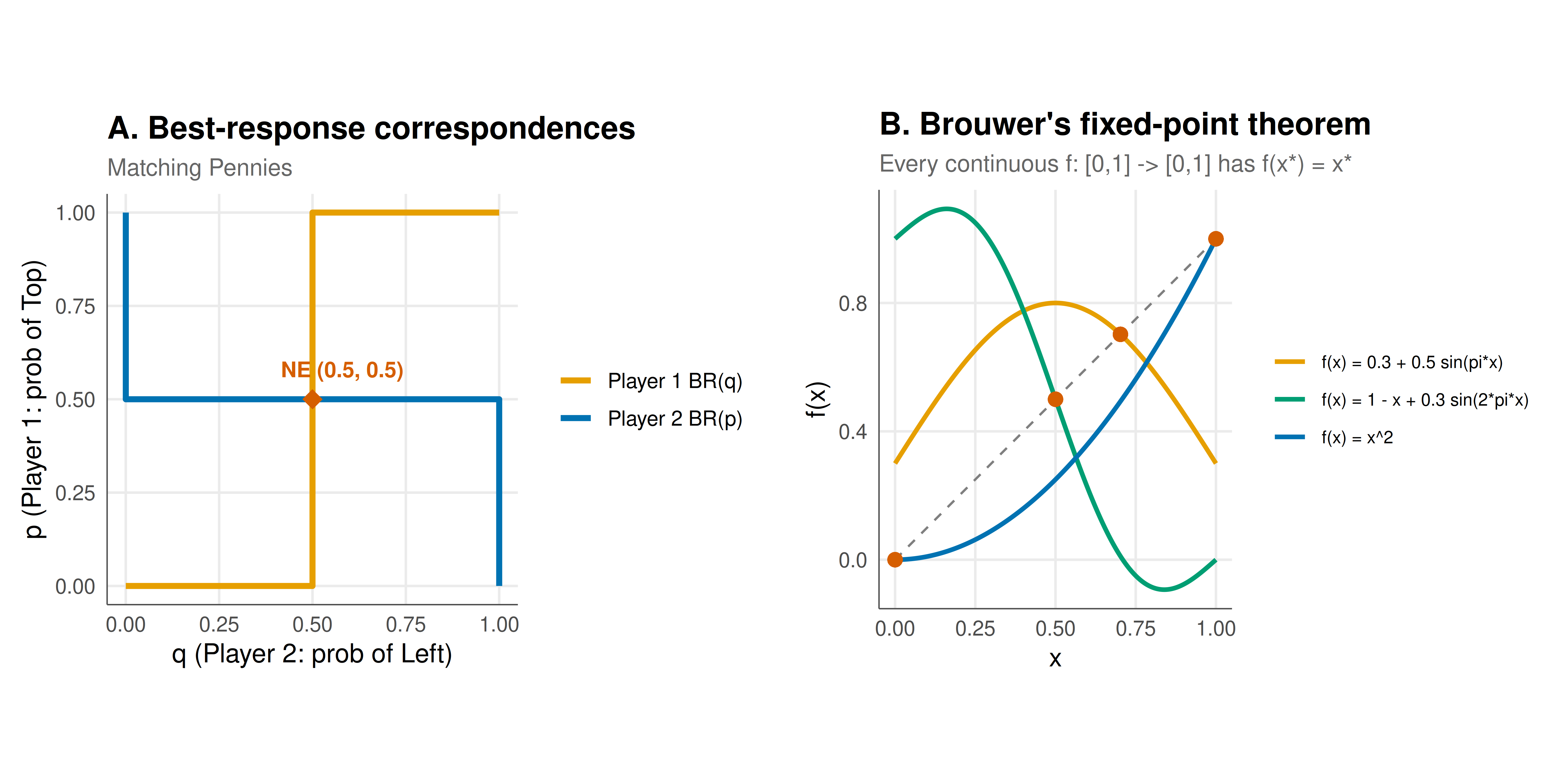
The figure shows two panels: (left) best-response correspondences for Matching Pennies with the unique mixed-strategy Nash equilibrium at their intersection, and (right) Brouwer's fixed-point theorem illustrated for three continuous functions on $[0,1]$.
```{r}
#| label: fig-nash-static
#| fig-cap: "Figure 1. Left: Best-response correspondences for Matching Pennies. Player 1's BR (orange) and Player 2's BR (blue) intersect at (p*, q*) = (0.5, 0.5), the unique mixed-strategy Nash equilibrium. Right: Brouwer's fixed-point theorem — every continuous function from [0,1] to [0,1] crosses the diagonal, guaranteeing a fixed point (red dots)."
#| dev: [png, pdf]
#| fig-width: 10
#| fig-height: 5
#| dpi: 300
# Panel A: Best responses for Matching Pennies
mp_br <- br_combined %>% filter(game == "Matching Pennies")
mp_ne <- ne_combined %>% filter(game == "Matching Pennies")

# For Matching Pennies, BR1 and BR2 are step functions
# BR1(q): if q > 0.5, p=1; if q < 0.5, p=0; if q=0.5, any p
# BR2(p): if p > 0.5, q=0; if p < 0.5, q=1; if p=0.5, any q

br1_segments <- tibble(
  x = c(0, 0.5, 0.5, 0.5, 1),
  y = c(0, 0, 0, 1, 1),
  player = "Player 1 BR(q)"
)
br2_segments <- tibble(
  x = c(1, 1, 0, 0, 0),
  y = c(0, 0.5, 0.5, 0.5, 1),
  player = "Player 2 BR(p)"
)

p_br <- ggplot() +
  geom_path(data = br1_segments, aes(x = x, y = y, colour = player), linewidth = 1.3) +
  geom_path(data = br2_segments, aes(x = x, y = y, colour = player), linewidth = 1.3) +
  geom_point(data = mp_ne, aes(x = q_ne, y = p_ne), colour = okabe_ito[6],
             size = 4, shape = 18) +
  annotate("text", x = mp_ne$q_ne[1] + 0.08, y = mp_ne$p_ne[1] + 0.08,
           label = "NE (0.5, 0.5)", colour = okabe_ito[6], size = 3.5, fontface = "bold") +
  scale_colour_manual(values = okabe_ito[c(1, 5)]) +
  coord_fixed() +
  labs(title = "A. Best-response correspondences",
       subtitle = "Matching Pennies",
       x = "q (Player 2: prob of Left)",
       y = "p (Player 1: prob of Top)",
       colour = NULL) +
  theme_publication() +
  theme(legend.position = "right")

# Panel B: Brouwer's theorem
p_brouwer <- ggplot() +
  geom_line(data = brouwer_data %>% filter(function_name == "f1") %>%
              select(x, y = diagonal) %>% distinct(),
            aes(x = x, y = y), linetype = "dashed", colour = "grey50", linewidth = 0.5) +
  geom_line(data = brouwer_data, aes(x = x, y = y, colour = function_label),
            linewidth = 1) +
  geom_point(data = fp_data, aes(x = x_fp, y = y_fp), colour = okabe_ito[6],
             size = 3, shape = 16) +
  scale_colour_manual(values = okabe_ito[c(1, 3, 5)]) +
  coord_fixed() +
  labs(title = "B. Brouwer's fixed-point theorem",
       subtitle = "Every continuous f: [0,1] -> [0,1] has f(x*) = x*",
       x = "x", y = "f(x)",
       colour = NULL) +
  theme_publication() +
  theme(legend.position = "right", legend.text = element_text(size = 8))

# Combine
gridExtra_available <- requireNamespace("gridExtra", quietly = TRUE)
if (gridExtra_available) {
  gridExtra::grid.arrange(p_br, p_brouwer, ncol = 2)
} else {
  p_br
}
```
## Interactive figure
Explore the Brouwer fixed-point illustration interactively. Hover over the curves to see function values and identify where each function crosses the diagonal.
```{r}
#| label: fig-nash-interactive
p_brouwer_int <- ggplot() +
  geom_line(data = brouwer_data %>% filter(function_name == "f1") %>%
              select(x, y = diagonal) %>% distinct(),
            aes(x = x, y = y), linetype = "dashed", colour = "grey50") +
  geom_line(data = brouwer_data,
            aes(x = x, y = y, colour = function_label,
                text = paste0("Function: ", function_label,
                              "\nx = ", round(x, 3),
                              "\nf(x) = ", round(y, 3),
                              "\nf(x) - x = ", round(y - x, 3))),
            linewidth = 0.9) +
  geom_point(data = fp_data,
             aes(x = x_fp, y = y_fp,
                 text = paste0("FIXED POINT\nx* = ", round(x_fp, 4))),
             colour = okabe_ito[6], size = 3) +
  scale_colour_manual(values = okabe_ito[c(1, 3, 5)]) +
  labs(title = "Brouwer's fixed-point theorem: interactive exploration",
       x = "x", y = "f(x)", colour = NULL) +
  theme_publication()

ggplotly(p_brouwer_int, tooltip = "text") %>%
  config(displaylogo = FALSE) %>%
  layout(legend = list(orientation = "h", y = -0.2))
```
## Interpretation
The visualisations bring Nash's abstract fixed-point argument to life. In the Matching Pennies game, the best-response correspondences form two step functions that intersect at exactly one point: $(p^*, q^*) = (0.5, 0.5)$. This is the unique Nash equilibrium, a mixed strategy where each player randomises uniformly. The geometric picture makes clear why this must be an equilibrium: at the intersection, each player is on their best-response curve simultaneously, so neither has an incentive to deviate.
For games with multiple equilibria (like the Battle of the Sexes), the best-response correspondences intersect at multiple points, including both pure-strategy equilibria and a mixed-strategy equilibrium. The Prisoner's Dilemma has a single intersection at a pure strategy (both defect), illustrating that the Nash equilibrium need not be efficient.
The Brouwer illustration provides the topological intuition behind existence. The diagonal $y = x$ divides the unit square, and any continuous function from $[0,1]$ to $[0,1]$ must cross it. This is because $f(0) \geq 0$ and $f(1) \leq 1$, so the function $g(x) = f(x) - x$ satisfies $g(0) \geq 0$ and $g(1) \leq 0$, and by the intermediate value theorem, $g(x^*) = 0$ for some $x^*$. The three functions in our illustration demonstrate that the fixed point can be unique (the sinusoidal function), at a boundary (the quadratic function has $f(0) = 0$), or in the interior (the decreasing function).
**Connection to computational complexity.** Nash's theorem guarantees existence but says nothing about how to *find* an equilibrium. In 2006, Daskalakis, Goldberg, and Papadimitriou proved that computing a Nash equilibrium is PPAD-complete --- a complexity class that captures problems where a solution is guaranteed to exist (by a parity argument) but finding it is believed to be computationally intractable. The Lemke-Howson algorithm [@lemke_howson_1964] can find Nash equilibria in two-player games by tracing paths on a labeled polytope, but its worst-case running time is exponential in the number of strategies. This is a remarkable situation in mathematics: we can *prove* that an object exists, yet (assuming standard complexity conjectures) no efficient algorithm can *find* it in general.
The historical context underscores the revolutionary nature of Nash's contribution. Von Neumann reportedly dismissed Nash's result as "trivial" --- a mere application of a fixed-point theorem [@von_neumann_morgenstern_1944]. But it was precisely this act of recognising that a fixed-point theorem could be applied to non-cooperative games that transformed game theory from a theory of zero-sum conflicts into a universal framework for strategic interaction. Nash's one-page proof [@nash_1950] and his fuller treatment in "Non-Cooperative Games" [@nash_1951] created the intellectual foundation on which modern economics, political science, evolutionary biology, and computer science now rest.
## Extensions & related tutorials
Nash's existence theorem is the starting point for virtually all of game theory. Understanding the proof connects to equilibrium refinements, computational methods, and applications across the site.
- [Tragedy of the commons](../../case-studies/tragedy-of-the-commons/) --- applying Nash equilibrium to an N-player commons game and comparing it with the social optimum
- [Difference-in-differences with strategic agents](../../causal-inference/difference-in-differences-strategic/) --- how Nash equilibrium shifts in response to policy create identification challenges
- [Zero-knowledge proofs](../../cryptography-and-gt/zero-knowledge-proofs/) --- PPAD-completeness of Nash equilibrium connects to computational complexity in cryptography
- [Dictator game and altruism](../../experimental-economics/dictator-game-altruism/) --- experimental departures from Nash predictions in the simplest possible game
## References
::: {#refs}
:::