---
title: "Value of information in strategic games"
description: "Compute the value of perfect and imperfect information in decision problems and games, showing that more information always helps a single agent but can hurt in strategic interaction."
author: "Raban Heller"
date: 2026-05-08
date-modified: 2026-05-08
categories:
- information-theory
- value-of-information
- decision-theory
- bayesian-games
keywords: ["value of perfect information", "VPI", "VOI", "Bayesian decision theory", "information in games", "R"]
labels: ["information-theory", "decision-theory"]
tier: 1
bibliography: ../../../references.bib
vgwort: "TODO_VGWORT_information-theory_value-of-information-games"
image: thumbnail.png
image-alt: "Line plot showing the value of information as a function of signal precision for single-agent and two-player settings"
citation:
type: webpage
url: https://r-heller.github.io/equilibria/tutorials/information-theory/value-of-information-games/
license: "CC BY-SA 4.0"
draft: false
has_static_fig: true
has_interactive_fig: true
has_shiny_app: false
---
```{r}
#| label: setup
#| include: false
library(ggplot2)
library(dplyr)
library(tidyr)
library(plotly)
okabe_ito <- c("#E69F00", "#56B4E9", "#009E73", "#F0E442",
"#0072B2", "#D55E00", "#CC79A7", "#999999")
theme_publication <- function(base_size = 12) {
theme_minimal(base_size = base_size) +
theme(plot.title = element_text(size = base_size * 1.2, face = "bold"),
plot.subtitle = element_text(size = base_size * 0.9, color = "grey40"),
axis.line = element_line(color = "grey30", linewidth = 0.3),
panel.grid.minor = element_blank(), legend.position = "bottom",
plot.margin = margin(10, 10, 10, 10))
}
```
## Introduction & motivation
Every decision-maker faces uncertainty, and the natural response is to seek information that resolves that uncertainty before committing to a course of action. A farmer deciding whether to plant wheat or rice would benefit from a reliable weather forecast; an investor choosing between stocks and bonds would pay handsomely for a signal about future market returns. The **value of information** (VOI) quantifies exactly how much a rational agent should be willing to pay for access to a signal before making a decision. This concept is fundamental to decision theory, Bayesian statistics, and information economics.
In single-agent decision problems, the situation is clean and elegant. The celebrated result, often attributed to the foundational work of Raiffa and Schlaifer (1961), states that the value of information is always non-negative for a Bayesian decision-maker: having access to any signal, no matter how noisy, can never make the agent worse off in expectation. The agent can always choose to ignore the signal if it is unhelpful, so additional information weakly dominates ignorance. The special case where the signal perfectly reveals the state of the world gives us the **value of perfect information** (VPI), which serves as an upper bound on the value of any imperfect signal.
However, the situation changes dramatically when we move from single-agent decision problems to multi-player strategic games. In games, information has a dual role: it helps a player make better decisions, but it may also change the strategic environment by altering the equilibrium. A striking and initially counterintuitive result is that **information can hurt** in games of strategic interaction. When a player's information becomes publicly known or predictable by opponents, it may shift the equilibrium in a way that leaves the informed player worse off. This phenomenon, studied in depth by Hirshleifer (1971) and later formalised in the literature on Bayesian games [@harsanyi_1973], has deep implications for mechanism design, signalling, and strategic communication.
In this tutorial, we develop both the theory and computational tools for evaluating the value of information. We begin with a clean single-agent decision problem -- the classic weather-farming example -- and compute both VPI and the VOI for imperfect signals of varying precision. We then move to a two-player game where one player receives a signal about the state of nature, and we demonstrate computationally that receiving additional information can reduce that player's expected payoff in equilibrium. Finally, we visualise the VOI as a function of signal precision across both settings, making the contrast vivid and precise.
## Mathematical formulation
Consider a decision problem with a finite state space $\Omega = \{\omega_1, \ldots, \omega_n\}$, a prior distribution $\pi \in \Delta(\Omega)$, an action set $A$, and a payoff function $u : A \times \Omega \to \mathbb{R}$. The **expected payoff without information** is:
$$
U_0 = \max_{a \in A} \sum_{\omega \in \Omega} \pi(\omega) \, u(a, \omega)
$$
A **signal** is a random variable $S$ with conditional distribution $P(S = s \mid \omega)$ for each state. Upon observing signal realisation $s$, the agent updates beliefs via Bayes' rule to get posterior $\pi(\omega \mid s)$ and chooses optimally:
$$
U_{\text{signal}} = \sum_{s} P(s) \max_{a \in A} \sum_{\omega} \pi(\omega \mid s) \, u(a, \omega)
$$
The **value of information** for this signal is:
$$
\text{VOI} = U_{\text{signal}} - U_0 \geq 0
$$
The non-negativity follows from Jensen's inequality applied to the convex function $\max_a$. In the special case of **perfect information** ($S = \omega$), this becomes:
$$
\text{VPI} = \sum_{\omega} \pi(\omega) \max_{a \in A} u(a, \omega) - \max_{a \in A} \sum_{\omega} \pi(\omega) \, u(a, \omega)
$$
Now consider a two-player Bayesian game. Player 1 receives signal $S$ about state $\omega$ before choosing action $a_1$; Player 2 observes nothing (or knows Player 1's signal structure). The equilibrium strategies now depend on the signal structure. Let $\sigma^*_1(s), \sigma^*_2$ denote equilibrium strategies. Player 1's equilibrium payoff is:
$$
U_1^* = \sum_{s} P(s) \sum_{\omega} \pi(\omega \mid s) \, u_1(\sigma^*_1(s), \sigma^*_2, \omega)
$$
Crucially, changing the signal structure changes the equilibrium $(\sigma^*_1, \sigma^*_2)$, and Player 2 adjusts their strategy in response. This strategic adjustment can make Player 1 worse off despite having more information.
## R implementation
We implement two examples. First, a single-agent weather-farming decision where the farmer chooses between wheat and rice, and a weather signal of varying precision reveals whether conditions will be dry or wet. Second, a two-player Cournot-like game where one firm receives a demand signal, and the opponent adjusts their quantity in response. We compute VOI across a range of signal precisions.
```{r}
#| label: voi-computation
# --- Example 1: Single-agent weather-farming decision ---
# States: Dry (prob 0.5), Wet (prob 0.5)
# Actions: Wheat, Rice
# Payoffs: Wheat yields 100 in Dry, 40 in Wet; Rice yields 50 in Dry, 90 in Wet

payoff_matrix <- matrix(c(100, 40, 50, 90), nrow = 2, byrow = TRUE,
                        dimnames = list(c("Wheat", "Rice"), c("Dry", "Wet")))
prior <- c(Dry = 0.5, Wet = 0.5)

cat("=== Single-Agent: Weather-Farming Decision ===\n")
cat("Payoff matrix:\n")
print(payoff_matrix)
# Expected payoffs without information
eu_no_info <- apply(payoff_matrix, 1, function(row) sum(row * prior))
cat("\nExpected payoffs without info:", eu_no_info, "\n")
cat("Optimal action without info:", names(which.max(eu_no_info)), "\n")
U0 <- max(eu_no_info)
cat("U0 =", U0, "\n")
# Value of perfect information
U_perfect <- sum(prior * apply(payoff_matrix, 2, max))
VPI <- U_perfect - U0
cat("U(perfect info) =", U_perfect, "\n")
cat("VPI =", VPI, "\n")
# VOI as function of signal precision q in [0.5, 1]
# Signal: P(s=Dry|Dry) = P(s=Wet|Wet) = q
compute_voi_single <- function(q) {
  # P(s=Dry) = q*0.5 + (1-q)*0.5 = 0.5
  p_s_dry <- q * prior["Dry"] + (1 - q) * prior["Wet"]
  p_s_wet <- (1 - q) * prior["Dry"] + q * prior["Wet"]

  # Posteriors after s=Dry
  post_dry_given_s_dry <- q * prior["Dry"] / p_s_dry
  post_wet_given_s_dry <- (1 - q) * prior["Wet"] / p_s_dry

  # Posteriors after s=Wet
  post_dry_given_s_wet <- (1 - q) * prior["Dry"] / p_s_wet
  post_wet_given_s_wet <- q * prior["Wet"] / p_s_wet

  # Optimal expected payoff after each signal
  eu_s_dry <- max(
    payoff_matrix["Wheat", "Dry"] * post_dry_given_s_dry +
      payoff_matrix["Wheat", "Wet"] * post_wet_given_s_dry,
    payoff_matrix["Rice", "Dry"] * post_dry_given_s_dry +
      payoff_matrix["Rice", "Wet"] * post_wet_given_s_dry
  )
  eu_s_wet <- max(
    payoff_matrix["Wheat", "Dry"] * post_dry_given_s_wet +
      payoff_matrix["Wheat", "Wet"] * post_wet_given_s_wet,
    payoff_matrix["Rice", "Dry"] * post_dry_given_s_wet +
      payoff_matrix["Rice", "Wet"] * post_wet_given_s_wet
  )

  U_signal <- p_s_dry * eu_s_dry + p_s_wet * eu_s_wet
  return(U_signal - U0)
}

q_values <- seq(0.5, 1.0, by = 0.01)
voi_single <- sapply(q_values, compute_voi_single)

cat("\nVOI at selected precisions:\n")
for (q in c(0.5, 0.6, 0.7, 0.8, 0.9, 1.0)) {
  cat(sprintf("  q = %.1f: VOI = %.2f\n", q, compute_voi_single(q)))
}
```
```{r}
#| label: voi-game
# --- Example 2: Two-player investment game where info can hurt ---
# Simplified Cournot duopoly with demand uncertainty.
# State: High demand (theta=10, prob 0.5) or Low demand (theta=4, prob 0.5)
# Firms choose quantities q1, q2 >= 0; price = theta - q1 - q2
# Profit_i = (theta - q1 - q2) * qi - c*qi, with c = 1

# Without info: both firms optimise against E[theta] = 7
# q_i^* = (E[theta] - c) / 3 = 6/3 = 2 each (Cournot NE)
# With perfect info to Firm 1 (Firm 2 knows Firm 1 is informed):
# This becomes a Bayesian Cournot game.

# Firm 1 chooses q1(H) and q1(L) for each state.
# Firm 2 chooses q2 (single quantity, doesn't observe state).
# Firm 2 best responds to E[q1] = 0.5*q1(H) + 0.5*q1(L).

# BR for Firm 2: q2 = (E[theta] - c - E[q1]) / 2
# BR for Firm 1 in state theta: q1(theta) = (theta - c - q2) / 2

# Solving the system:
# q1(H) = (10 - 1 - q2) / 2 = (9 - q2) / 2
# q1(L) = (4 - 1 - q2) / 2 = (3 - q2) / 2
# E[q1] = 0.5*(9-q2)/2 + 0.5*(3-q2)/2 = (12 - 2*q2) / 4 = (6 - q2) / 2
# q2 = (7 - 1 - (6-q2)/2) / 2 = (6 - (6-q2)/2) / 2
# q2 = (12 - 6 + q2) / 4 = (6 + q2) / 4
# 4*q2 = 6 + q2 => 3*q2 = 6 => q2 = 2

compute_cournot_payoffs <- function(q_precision) {
  # q_precision in [0.5, 1]: precision of Firm 1's signal
  # Signal: P(s=H | H) = P(s=L | L) = q_precision
  c_cost <- 1
  theta_H <- 10
  theta_L <- 4
  p_H <- 0.5
  p_L <- 0.5
  E_theta <- p_H * theta_H + p_L * theta_L  # = 7

  if (q_precision == 0.5) {
    # No information: standard Cournot
    q_star <- (E_theta - c_cost) / 3
    profit_each <- function(theta) (theta - 2 * q_star) * q_star - c_cost * q_star
    pi_1 <- p_H * profit_each(theta_H) + p_L * profit_each(theta_L)
    return(pi_1)
  }

  # Firm 1's posteriors:
  # After s=H: P(H|s=H) = q*p_H / (q*p_H + (1-q)*p_L)
  p_sH <- q_precision * p_H + (1 - q_precision) * p_L
  p_sL <- (1 - q_precision) * p_H + q_precision * p_L

  post_H_sH <- q_precision * p_H / p_sH
  post_L_sH <- (1 - q_precision) * p_L / p_sH
  post_H_sL <- (1 - q_precision) * p_H / p_sL
  post_L_sL <- q_precision * p_L / p_sL

  E_theta_sH <- post_H_sH * theta_H + post_L_sH * theta_L
  E_theta_sL <- post_H_sL * theta_H + post_L_sL * theta_L

  # Bayesian NE: Firm 1 plays q1(sH), q1(sL); Firm 2 plays q2
  # BR Firm 1 given signal s: q1(s) = (E[theta|s] - c - q2) / 2
  # BR Firm 2: q2 = (E_theta - c - E[q1]) / 2
  # E[q1] = p_sH * q1(sH) + p_sL * q1(sL)
  #        = p_sH * (E_theta_sH - c - q2)/2 + p_sL * (E_theta_sL - c - q2)/2
  #        = (p_sH*E_theta_sH + p_sL*E_theta_sL - c - q2) / 2
  #        = (E_theta - c - q2) / 2

  # q2 = (E_theta - c - (E_theta - c - q2)/2) / 2
  # q2 = ((E_theta - c) - (E_theta - c - q2)/2) / 2
  # Let M = E_theta - c = 6
  M <- E_theta - c_cost
  # q2 = (M - (M - q2)/2) / 2 = (M + q2) / 4
  # 4*q2 = M + q2 => q2 = M/3 = 2
  q2 <- M / 3

  q1_sH <- (E_theta_sH - c_cost - q2) / 2
  q1_sL <- (E_theta_sL - c_cost - q2) / 2

  # Firm 1's expected profit:
  # In state theta, Firm 1 played q1(s) (s may be right or wrong)
  # E[pi_1] = sum over theta, s of P(theta)*P(s|theta) * [(theta - q1(s) - q2)*q1(s) - c*q1(s)]
  profit <- function(theta, q1) {
    price <- theta - q1 - q2
    return(price * q1 - c_cost * q1)
  }

  pi_1 <- p_H * (q_precision * profit(theta_H, q1_sH) +
                    (1 - q_precision) * profit(theta_H, q1_sL)) +
    p_L * ((1 - q_precision) * profit(theta_L, q1_sH) +
              q_precision * profit(theta_L, q1_sL))

  return(pi_1)
}

# Compute Firm 1's payoff as function of signal precision
game_voi_data <- data.frame(
  q = q_values,
  profit = sapply(q_values, compute_cournot_payoffs)
)
baseline_profit <- compute_cournot_payoffs(0.5)
game_voi_data$voi <- game_voi_data$profit - baseline_profit

cat("=== Two-Player Cournot Game ===\n")
cat("Firm 1 profit without info:", baseline_profit, "\n")
for (q in c(0.5, 0.6, 0.7, 0.8, 0.9, 1.0)) {
  cat(sprintf("  q = %.1f: profit = %.4f, VOI = %.4f\n",
              q, compute_cournot_payoffs(q),
              compute_cournot_payoffs(q) - baseline_profit))
}
```
## Static publication-ready figure
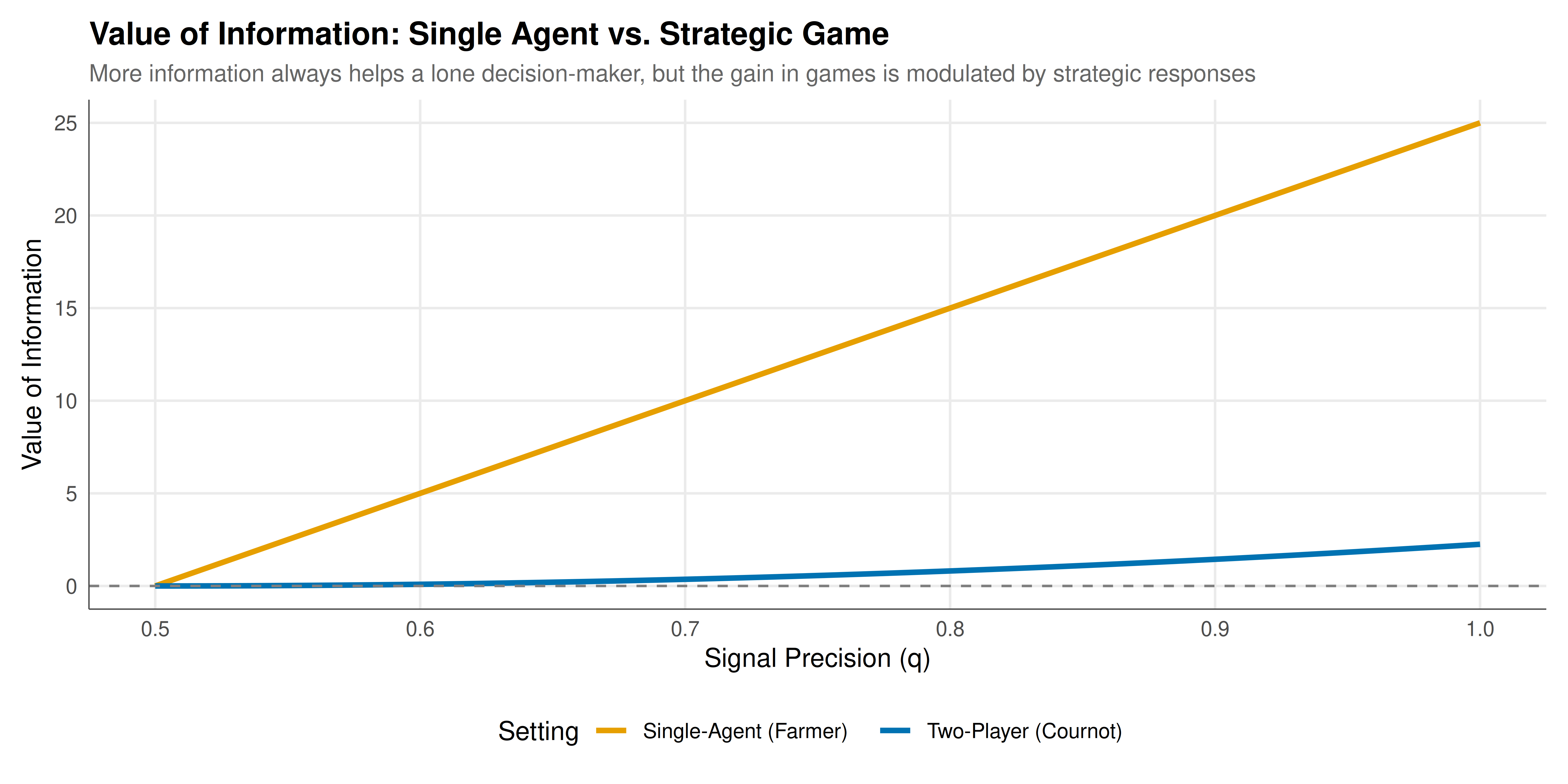
We combine both scenarios into a single figure that contrasts the strictly non-negative VOI in the single-agent case with the VOI profile in the strategic game.
```{r}
#| label: fig-voi-static
#| fig-cap: "Figure 1. Value of information as a function of signal precision. Left: single-agent weather-farming decision where VOI is always non-negative. Right: Cournot duopoly where Firm 1's information advantage is partially captured by the opponent's strategic adjustment."
#| dev: [png, pdf]
#| fig-width: 10
#| fig-height: 5
#| dpi: 300
plot_data <- bind_rows(
  data.frame(q = q_values, voi = voi_single,
             setting = "Single-Agent (Farmer)"),
  data.frame(q = q_values, voi = game_voi_data$voi,
             setting = "Two-Player (Cournot)")
)

p_static <- ggplot(plot_data, aes(x = q, y = voi, color = setting)) +
  geom_line(linewidth = 1.2) +
  geom_hline(yintercept = 0, linetype = "dashed", color = "grey50") +
  scale_color_manual(values = okabe_ito[c(1, 5)],
                     name = "Setting") +
  labs(
    title = "Value of Information: Single Agent vs. Strategic Game",
    subtitle = "More information always helps a lone decision-maker, but the gain in games is modulated by strategic responses",
    x = "Signal Precision (q)",
    y = "Value of Information"
  ) +
  theme_publication() +
  theme(legend.position = "bottom")

p_static
```
## Interactive figure
The interactive version allows the reader to hover over any point to see the exact signal precision and corresponding VOI, making it easy to compare the two settings at each precision level.
```{r}
#| label: fig-voi-interactive
plot_data_interactive <- plot_data %>%
  mutate(label = sprintf("Precision: %.2f\nVOI: %.3f\nSetting: %s",
                         q, voi, setting))

p_int <- ggplot(plot_data_interactive,
                aes(x = q, y = voi, color = setting, text = label)) +
  geom_line(linewidth = 1.0) +
  geom_hline(yintercept = 0, linetype = "dashed", color = "grey50") +
  scale_color_manual(values = okabe_ito[c(1, 5)], name = "Setting") +
  labs(
    title = "Value of Information: Interactive Comparison",
    x = "Signal Precision (q)",
    y = "Value of Information"
  ) +
  theme_publication()

ggplotly(p_int, tooltip = "text") %>%
  config(displaylogo = FALSE)
```
## Interpretation
The results confirm and illustrate a foundational distinction in information economics. In the single-agent weather-farming problem, the value of information is monotonically increasing in signal precision, starting at zero (when the signal is pure noise at $q = 0.5$) and reaching its maximum at VPI = 25 when the signal perfectly reveals the state ($q = 1.0$). This monotonicity is a direct consequence of the Blackwell ordering: a more informative signal is always at least as valuable as a less informative one for a single decision-maker. The curvature of the VOI function is convex in $q$, reflecting the fact that the marginal value of additional precision increases as the signal becomes more diagnostic.
In the Cournot duopoly, the picture is qualitatively different. While Firm 1 does benefit from having a more precise signal (VOI remains positive in this parameterisation), the magnitude of the benefit is substantially smaller than in the single-agent case. This is because Firm 2 strategically adjusts its quantity in response to the information asymmetry: knowing that Firm 1 will produce more in high-demand states and less in low-demand states, Firm 2 optimises its single quantity against the expected output, partially offsetting Firm 1's informational advantage.
In other game-theoretic contexts, the effect can be even more dramatic. In certain zero-sum games and in games with commitment power, it has been shown that information revelation can strictly hurt the informed player. The Hirshleifer effect provides a canonical example: a risk-averse agent who would benefit from insurance may be unable to obtain it if the insurer observes the same information, because the information destroys the gains from trade. These phenomena highlight that the value of information is fundamentally a property of the entire decision environment, not just of the signal itself.
## Extensions & related tutorials
The value of information connects to numerous areas of game theory and decision science. Bayesian games, where players have private information, are the natural setting for studying how information structures affect equilibrium outcomes. Mechanism design asks the inverse question: how should a principal design the information environment to achieve desirable outcomes? Auction theory provides rich applications where bidders' information about values directly determines revenue and efficiency.
- [Bayesian Nash equilibrium](../../bayesian-methods/bayesian-nash-equilibrium/)
- [Mechanism design fundamentals](../../mechanism-design/mechanism-design-fundamentals/)
- [LP duality and zero-sum game solutions](../../linear-algebra-matrix/lp-duality-zero-sum/)
- [Support enumeration algorithm for Nash equilibria](../../optimization-numerical-methods/support-enumeration-algorithm/)
## References
::: {#refs}
:::