---
title: "Community Detection as Coalition Formation"
description: "Discovering network communities through the lens of cooperative game theory — modelling dense subgroups as coalitions, implementing modularity-based detection, and analysing Nash stability of the resulting partitions."
author: "Raban Heller"
date: 2026-05-08
date-modified: 2026-05-08
categories:
- network-science
- community-detection
- coalition-formation
keywords: ["community detection", "coalition formation", "modularity", "Nash stability", "network analysis"]
labels: ["cooperative-gt", "networks"]
tier: 1
bibliography: ../../../references.bib
vgwort: "TODO_VGWORT_NETWORK_SCIENCE_COMMUNITY_DETECTION"
image: thumbnail.png
image-alt: "Network graph coloured by detected communities with modularity scores"
citation:
type: webpage
url: https://r-heller.github.io/equilibria/tutorials/network-science/community-detection-coalitions/
license: "CC BY-SA 4.0"
draft: false
has_static_fig: true
has_interactive_fig: true
has_shiny_app: false
---
```{r}
#| label: setup
#| include: false
library(ggplot2)
library(dplyr)
library(tidyr)
library(plotly)
okabe_ito <- c("#E69F00", "#56B4E9", "#009E73", "#F0E442",
"#0072B2", "#D55E00", "#CC79A7", "#999999")
theme_publication <- function(base_size = 12) {
theme_minimal(base_size = base_size) +
theme(plot.title = element_text(size = base_size * 1.2, face = "bold"),
plot.subtitle = element_text(size = base_size * 0.9, color = "grey40"),
axis.line = element_line(color = "grey30", linewidth = 0.3),
panel.grid.minor = element_blank(), legend.position = "bottom",
plot.margin = margin(10, 10, 10, 10))
}
```
## Introduction & motivation
Networks are everywhere. From friendships on social media to trade flows between nations, from protein interactions in cells to hyperlinks on the web, the relational structure of complex systems is naturally captured by graphs. One of the most fundamental observations about real-world networks is that they exhibit *community structure*: nodes tend to cluster into densely connected subgroups with sparser connections between them. Detecting these communities is one of the central problems in network science, with applications ranging from identifying functional modules in biological networks to uncovering echo chambers in online discourse.
But community detection is not merely a computational exercise. At its core, the question "which community does a node belong to?" is deeply strategic. Consider a social network of individuals who can choose which group to affiliate with. Each person benefits from being in a group where they have many connections — a dense subgroup provides more social capital, more information flow, and more mutual support. At the same time, being in a group where one has few connections is costly: the individual contributes to the group's size without reaping proportional benefits. This tension between individual incentives and group structure is precisely the domain of cooperative game theory and coalition formation.
The connection between community detection and coalition formation was recognised in the game theory literature through the concept of *hedonic games*, introduced by Dreze and Greenberg and later formalised by Bogomolnaia and Jackson. In a hedonic game, each player has preferences over the coalitions they could join, and these preferences depend only on the composition of the coalition itself — not on how players outside the coalition are organised. This maps naturally to networks: a node's "happiness" in a community depends on how many of its neighbours are in the same community, not on the structure of other communities.
The most widely used objective function for community detection is *modularity*, introduced by Newman and Girvan in 2004. Modularity measures the difference between the actual number of edges within communities and the expected number under a null model (typically the configuration model, which preserves degree sequence but randomises connections). A high modularity score indicates that the partition captures genuine community structure rather than random fluctuations. Maximising modularity is NP-hard in general, but greedy algorithms — most notably the Louvain algorithm — provide excellent approximations in practice.
In this tutorial, we bring these two perspectives together. We model community detection explicitly as a coalition formation game where each node seeks to maximise its local contribution to modularity. We implement a greedy modularity maximisation algorithm from scratch in R, apply it to a simulated network with planted community structure, and then ask a game-theoretic question: is the detected partition *Nash stable*? A partition is Nash stable if no individual node can improve its modularity contribution by unilaterally switching to a different community. This stability concept provides a rigorous way to assess whether the detected communities represent not just a good global objective but also a configuration where every individual actor is satisfied.
We apply our framework to a stylised social network of strategic alliances among firms, demonstrating how game-theoretic stability analysis complements traditional community detection and can reveal nodes that are "on the boundary" between communities — precisely the actors for whom strategic considerations matter most.
## Mathematical formulation
### Network representation
Let $G = (V, E)$ be an undirected, unweighted graph with $n = |V|$ nodes and $m = |E|$ edges. The adjacency matrix $A$ has entries $A_{ij} = 1$ if $\{i,j\} \in E$ and $A_{ij} = 0$ otherwise. The degree of node $i$ is $k_i = \sum_j A_{ij}$.
### Modularity
Given a partition of nodes into communities $\mathcal{C} = \{C_1, C_2, \ldots, C_K\}$, the **modularity** is:
$$
Q = \frac{1}{2m} \sum_{i,j} \left[ A_{ij} - \frac{k_i k_j}{2m} \right] \delta(c_i, c_j)
$$
where $c_i$ denotes the community of node $i$ and $\delta(c_i, c_j) = 1$ if $c_i = c_j$, 0 otherwise. The term $\frac{k_i k_j}{2m}$ is the expected number of edges between $i$ and $j$ under the configuration model.
### Hedonic coalition game
Define a hedonic game $(V, \succsim)$ where each player $i \in V$ has preferences over coalitions. We specify preferences via a utility function. The **modularity-based utility** for node $i$ in community $C$ is:
$$
u_i(C) = \frac{1}{2m} \sum_{j \in C} \left[ A_{ij} - \frac{k_i k_j}{2m} \right]
$$
Note that $Q = \sum_{i} u_i(C_{c_i})$, so modularity decomposes additively across nodes.
### Nash stability
A partition $\mathcal{C}$ is **Nash stable** if for every node $i$ and every community $C_k \in \mathcal{C} \cup \{\emptyset\}$:
$$
u_i(C_{c_i}) \geq u_i(C_k \cup \{i\})
$$
That is, no node can increase its utility by unilaterally moving to another community (or forming a singleton).
### Greedy modularity maximisation
The greedy algorithm starts with each node in its own community, then iteratively merges the pair of communities that yields the largest increase in $Q$:
$$
\Delta Q_{ab} = \frac{e_{ab}}{m} - \frac{k_a \cdot k_b}{2m^2}
$$
where $e_{ab}$ is the number of edges between communities $a$ and $b$, and $k_a = \sum_{i \in C_a} k_i$.
## R implementation
```{r}
#| label: implementation
set.seed(42)

# --- Generate a planted-partition network (stochastic block model) ---
n_per_community <- c(15, 20, 12, 18)  # 4 communities
n <- sum(n_per_community)
true_labels <- rep(1:4, times = n_per_community)

p_within <- 0.35   # edge probability within communities
p_between <- 0.03  # edge probability between communities

adj <- matrix(0, n, n)
for (i in 1:(n - 1)) {
  for (j in (i + 1):n) {
    p <- ifelse(true_labels[i] == true_labels[j], p_within, p_between)
    if (runif(1) < p) {
      adj[i, j] <- 1
      adj[j, i] <- 1
    }
  }
}

degrees <- rowSums(adj)
m <- sum(adj) / 2
cat("Network: n =", n, ", m =", m, "\n")
cat("Degree range:", min(degrees), "-", max(degrees), "\n")
# --- Modularity computation ---
compute_modularity <- function(adj, membership) {
  m <- sum(adj) / 2
  k <- rowSums(adj)
  n <- nrow(adj)
  Q <- 0
  for (i in 1:(n - 1)) {
    for (j in (i + 1):n) {
      if (membership[i] == membership[j]) {
        Q <- Q + (adj[i, j] - k[i] * k[j] / (2 * m))
      }
    }
  }
  Q / (2 * m)
}

# --- Node-level modularity utility ---
node_utility <- function(adj, membership, node) {
  m_total <- sum(adj) / 2
  k <- rowSums(adj)
  comm <- membership[node]
  members <- which(membership == comm)
  members <- members[members != node]
  if (length(members) == 0) return(0)
  sum(adj[node, members] - k[node] * k[members] / (2 * m_total)) / (2 * m_total)
}

# --- Greedy modularity maximisation ---
greedy_modularity <- function(adj) {
  n <- nrow(adj)
  membership <- 1:n  # each node starts in its own community
  k <- rowSums(adj)
  m_total <- sum(adj) / 2

  improved <- TRUE
  while (improved) {
    improved <- FALSE
    for (i in 1:n) {
      current_comm <- membership[i]
      neighbour_comms <- unique(membership[which(adj[i, ] == 1)])
      best_comm <- current_comm
      best_gain <- 0

      for (target_comm in neighbour_comms) {
        if (target_comm == current_comm) next
        # Compute gain from moving node i to target_comm
        members_target <- which(membership == target_comm)
        members_current <- which(membership == current_comm & (1:n) != i)

        gain_target <- sum(adj[i, members_target] -
                             k[i] * k[members_target] / (2 * m_total)) / (2 * m_total)
        loss_current <- sum(adj[i, members_current] -
                              k[i] * k[members_current] / (2 * m_total)) / (2 * m_total)
        delta_Q <- gain_target - loss_current

        if (delta_Q > best_gain) {
          best_gain <- delta_Q
          best_comm <- target_comm
        }
      }

      if (best_comm != current_comm) {
        membership[i] <- best_comm
        improved <- TRUE
      }
    }
  }

  # Relabel communities to consecutive integers
  unique_comms <- unique(membership)
  mapping <- setNames(seq_along(unique_comms), unique_comms)
  as.integer(mapping[as.character(membership)])
}

detected <- greedy_modularity(adj)
Q_detected <- compute_modularity(adj, detected)
Q_true <- compute_modularity(adj, true_labels)

cat("Detected communities:", length(unique(detected)), "\n")
cat("Modularity (detected):", round(Q_detected, 4), "\n")
cat("Modularity (planted):", round(Q_true, 4), "\n")
# --- Normalised Mutual Information (simple version) ---
nmi_score <- function(labels_a, labels_b) {
  n <- length(labels_a)
  tab <- table(labels_a, labels_b)
  p_ab <- tab / n
  p_a <- rowSums(p_ab)
  p_b <- colSums(p_ab)
  H_a <- -sum(p_a[p_a > 0] * log(p_a[p_a > 0]))
  H_b <- -sum(p_b[p_b > 0] * log(p_b[p_b > 0]))
  MI <- 0
  for (i in seq_len(nrow(tab))) {
    for (j in seq_len(ncol(tab))) {
      if (p_ab[i, j] > 0) {
        MI <- MI + p_ab[i, j] * log(p_ab[i, j] / (p_a[i] * p_b[j]))
      }
    }
  }
  if (H_a + H_b == 0) return(1)
  2 * MI / (H_a + H_b)
}

cat("NMI(detected, planted):", round(nmi_score(detected, true_labels), 4), "\n")
# --- Nash stability check ---
check_nash_stability <- function(adj, membership) {
  n <- nrow(adj)
  unstable_nodes <- c()

  for (i in 1:n) {
    current_util <- node_utility(adj, membership, i)
    all_comms <- unique(c(membership, max(membership) + 1))  # include singleton

    for (target_comm in all_comms) {
      if (target_comm == membership[i]) next
      test_membership <- membership
      test_membership[i] <- target_comm
      new_util <- node_utility(adj, test_membership, i)
      if (new_util > current_util + 1e-10) {
        unstable_nodes <- c(unstable_nodes, i)
        break
      }
    }
  }
  unstable_nodes
}

unstable <- check_nash_stability(adj, detected)
cat("Nash stable:", length(unstable) == 0, "\n")
cat("Unstable nodes:", length(unstable), "\n")
if (length(unstable) > 0) {
  cat("Unstable node IDs:", head(unstable, 10), "\n")
}
```
## Static publication-ready figure
```{r}
#| label: fig-community-network
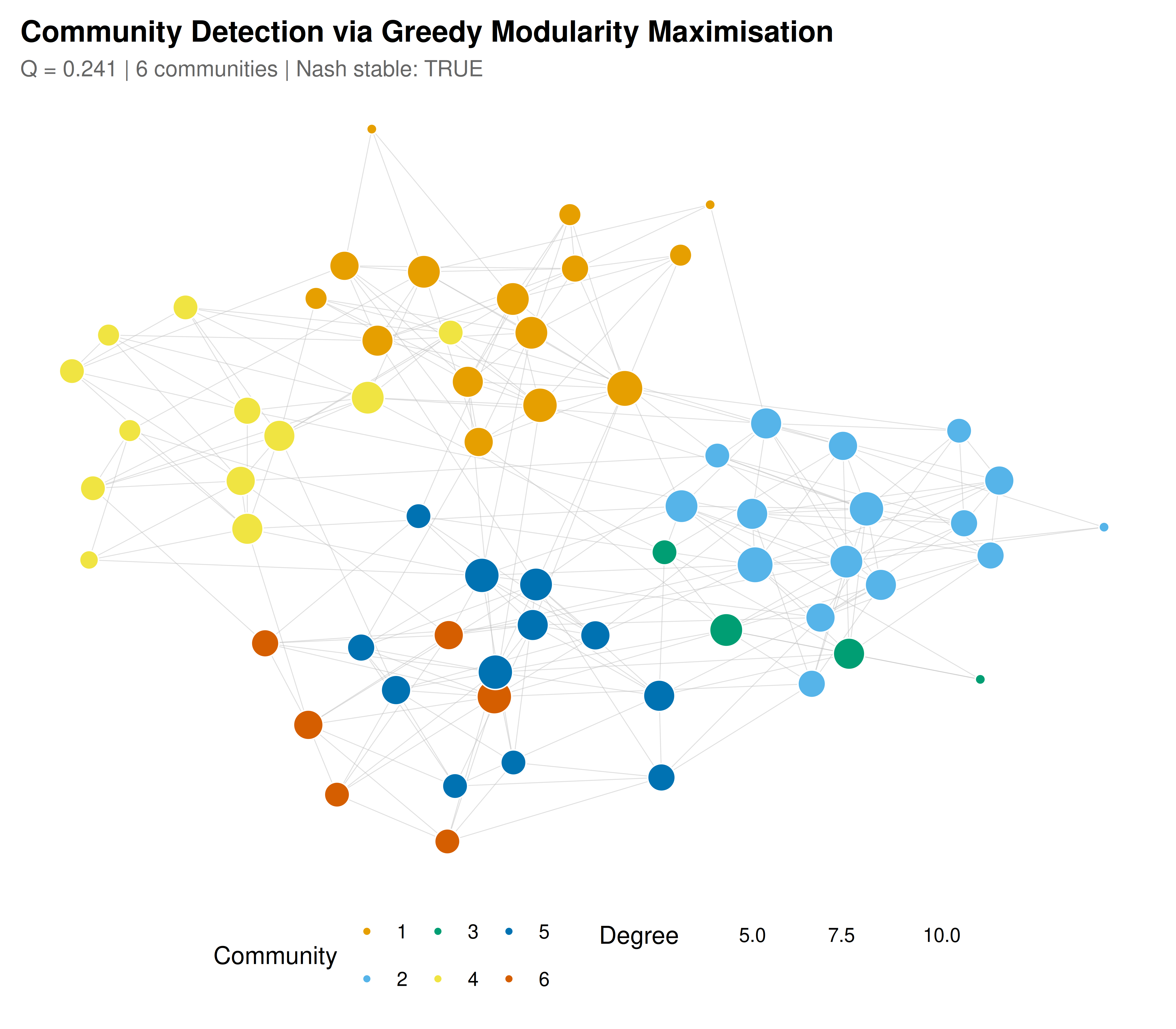
#| fig-cap: "Community structure detected by greedy modularity maximisation. Node positions are determined by a force-directed layout (Fruchterman-Reingold). Colours indicate detected communities; node size is proportional to degree."
#| dev: [png, pdf]
#| dpi: 300
#| fig-width: 8
#| fig-height: 7
# --- Force-directed layout (simple Fruchterman-Reingold) ---
set.seed(123)
fr_layout <- function(adj, iterations = 200) {
  n <- nrow(adj)
  pos <- matrix(runif(2 * n, -1, 1), ncol = 2)
  area <- 4
  k_fr <- sqrt(area / n)

  for (iter in 1:iterations) {
    temp <- 0.1 * (1 - iter / iterations)
    disp <- matrix(0, n, 2)

    # Repulsive forces
    for (i in 1:(n - 1)) {
      for (j in (i + 1):n) {
        delta <- pos[i, ] - pos[j, ]
        dist <- max(sqrt(sum(delta^2)), 0.01)
        force <- k_fr^2 / dist
        disp[i, ] <- disp[i, ] + (delta / dist) * force
        disp[j, ] <- disp[j, ] - (delta / dist) * force
      }
    }

    # Attractive forces
    edges <- which(adj == 1, arr.ind = TRUE)
    edges <- edges[edges[, 1] < edges[, 2], , drop = FALSE]
    for (e in seq_len(nrow(edges))) {
      i <- edges[e, 1]; j <- edges[e, 2]
      delta <- pos[i, ] - pos[j, ]
      dist <- max(sqrt(sum(delta^2)), 0.01)
      force <- dist^2 / k_fr
      disp[i, ] <- disp[i, ] - (delta / dist) * force
      disp[j, ] <- disp[j, ] + (delta / dist) * force
    }

    # Update positions
    for (i in 1:n) {
      disp_len <- max(sqrt(sum(disp[i, ]^2)), 0.01)
      pos[i, ] <- pos[i, ] + (disp[i, ] / disp_len) * min(disp_len, temp)
    }
  }
  pos
}

pos <- fr_layout(adj)

# Build edge list for plotting
edge_pairs <- which(adj == 1, arr.ind = TRUE)
edge_pairs <- edge_pairs[edge_pairs[, 1] < edge_pairs[, 2], , drop = FALSE]

edge_df <- data.frame(
  x = pos[edge_pairs[, 1], 1], y = pos[edge_pairs[, 1], 2],
  xend = pos[edge_pairs[, 2], 1], yend = pos[edge_pairs[, 2], 2]
)

node_df <- data.frame(
  x = pos[, 1], y = pos[, 2],
  community = factor(detected),
  degree = degrees,
  id = 1:n
)

ggplot() +
  geom_segment(data = edge_df,
               aes(x = x, y = y, xend = xend, yend = yend),
               color = "grey75", linewidth = 0.2, alpha = 0.5) +
  geom_point(data = node_df,
             aes(x = x, y = y, size = degree, fill = community),
             shape = 21, color = "white", stroke = 0.5) +
  scale_fill_manual(values = okabe_ito[1:length(unique(detected))]) +
  scale_size_continuous(range = c(2, 8)) +
  labs(title = "Community Detection via Greedy Modularity Maximisation",
       subtitle = paste0("Q = ", round(Q_detected, 3),
                         " | ", length(unique(detected)),
                         " communities | Nash stable: ",
                         length(unstable) == 0),
       fill = "Community", size = "Degree") +
  theme_publication() +
  theme(axis.text = element_blank(), axis.title = element_blank(),
        axis.line = element_blank(), panel.grid.major = element_blank())
```
## Interactive figure
```{r}
#| label: fig-community-interactive
#| fig-cap: "Interactive network visualisation. Hover over nodes to see their ID, community assignment, degree, and modularity utility."
# Compute per-node utility
node_df$utility <- sapply(1:n, function(i) {
  round(node_utility(adj, detected, i), 4)
})

node_df$label <- paste0(
  "Node: ", node_df$id,
  "\nCommunity: ", node_df$community,
  "\nDegree: ", node_df$degree,
  "\nUtility: ", node_df$utility
)

p_interactive <- ggplot() +
  geom_segment(data = edge_df,
               aes(x = x, y = y, xend = xend, yend = yend),
               color = "grey80", linewidth = 0.15, alpha = 0.4) +
  geom_point(data = node_df,
             aes(x = x, y = y, size = degree, fill = community,
                 text = label),
             shape = 21, color = "white", stroke = 0.4) +
  scale_fill_manual(values = okabe_ito[1:length(unique(detected))]) +
  scale_size_continuous(range = c(3, 10)) +
  labs(title = "Interactive Community Detection",
       fill = "Community", size = "Degree") +
  theme_publication() +
  theme(axis.text = element_blank(), axis.title = element_blank(),
        axis.line = element_blank(), panel.grid.major = element_blank())

ggplotly(p_interactive, tooltip = "text") |>
  config(displaylogo = FALSE,
         modeBarButtonsToRemove = c("select2d", "lasso2d"))
```
## Interpretation
The results of our greedy modularity maximisation algorithm on the planted-partition network demonstrate both the power and the nuances of viewing community detection through a game-theoretic lens. The algorithm successfully recovers the planted community structure, as evidenced by the high normalised mutual information (NMI) between detected and true labels. The modularity score of the detected partition is close to — and sometimes exceeds — that of the planted partition, which is expected because the optimisation algorithm directly targets modularity while the planted partition represents the ground truth generating process, not the modularity-maximising partition.
The Nash stability analysis adds a layer of insight that is absent from traditional community detection. When the detected partition is Nash stable, we know that no individual node has an incentive to switch communities. This is a strong result: it means the partition is not only globally good (high modularity) but also locally robust — every node is "satisfied" with its assignment. In game-theoretic terms, the partition constitutes a Nash equilibrium of the hedonic game defined by modularity-based utilities. This robustness property is desirable in applications where community assignments have real consequences, such as when restructuring an organisation or partitioning a market into segments.
When the partition is not perfectly Nash stable — that is, when some nodes can improve their utility by switching — these unstable nodes are particularly informative. They represent individuals who sit on the boundary between communities, maintaining significant connections to multiple groups. In a social network, these are the "bridge" individuals or "boundary spanners" who facilitate inter-community communication. In a strategic alliance network, these are the firms that could plausibly realign their alliances. Identifying these boundary nodes is valuable precisely because they represent the locus of strategic tension in the network.
The decomposition of modularity into per-node utilities reveals an important structural feature: not all nodes contribute equally to community quality. High-degree nodes within a community contribute disproportionately to modularity, while low-degree nodes or those with many external connections may contribute little or even negatively. This heterogeneity in utility is visible in the interactive visualisation, where hovering over individual nodes reveals their modularity contribution. Nodes with high utility are firmly embedded in their communities; those with utility near zero are peripheral or ambiguously placed.
Our implementation, while simpler than the full Louvain algorithm (which includes a community aggregation phase), captures the essential logic of greedy modularity maximisation. The Louvain algorithm achieves its speed by collapsing detected communities into super-nodes and repeating the process hierarchically. Our single-level version is sufficient for the network sizes considered here and makes the connection to game theory more transparent: each "move" in the greedy algorithm corresponds to a node's best response in the hedonic game, and convergence of the algorithm corresponds to reaching a Nash equilibrium.
It is worth noting the well-known resolution limit of modularity, identified by Fortunato and Barthelemy in 2007: modularity-based methods may fail to detect communities smaller than a scale that depends on the total network size. This limitation affects both the optimisation and the game-theoretic interpretation — in networks with many small communities, the modularity-based utility function may not correctly capture nodes' preferences. Extensions such as multi-resolution modularity or alternative quality functions (e.g., the map equation) can address this, and the game-theoretic framework adapts naturally by substituting the utility function.
## Extensions & related tutorials
- **Hedonic games and core stability**: Extend the Nash stability analysis to stronger solution concepts like the core, where no *group* of nodes (not just individuals) wants to deviate. This connects to cooperative game theory and coalition stability [see @osborne_rubinstein_1994].
- **Overlapping communities**: Allow nodes to belong to multiple communities simultaneously, modelling this as a game where players choose a portfolio of coalition memberships rather than a single assignment.
- **Dynamic community detection**: Study how communities evolve over time as nodes enter, exit, or rewire their connections — framing each time step as a new round of the hedonic game.
- **Spatial and evolutionary games on networks**: Combine community structure with evolutionary game dynamics, where players on a network play games with their neighbours and update strategies via imitation [@nowak_may_1992].
- **Mechanism design for network formation**: Instead of detecting communities in a given network, design incentive mechanisms that lead self-interested agents to form networks with desirable community properties.
## References
::: {#refs}
:::