VAR Models for Strategic Interaction Dynamics

Vector autoregression models capture dynamic strategic interdependence in oligopoly markets, revealing how firms’ quantities today depend on rivals’ past decisions through impulse response functions and Granger causality tests.

Keywords

vector autoregression, VAR, Granger causality, impulse response function, strategic interaction, duopoly, Cournot, R

Introduction & motivation

Classical game theory models strategic interaction as a one-shot or static phenomenon. In the canonical Cournot duopoly, two firms simultaneously choose quantities, and the Nash equilibrium is computed from the intersection of best-response functions at a single point in time. This framework has enormous explanatory power, but it abstracts away a crucial feature of real-world competition: firms interact repeatedly over time, and their decisions today are shaped by what their rivals did yesterday, last quarter, and last year. The static Nash equilibrium tells us where the system might rest, but it says nothing about the dynamic path firms follow to get there, how they respond to shocks, or whether one firm’s strategy adjustments systematically lead or follow the other’s.

Vector autoregression (VAR) models, introduced to macroeconomics by Christopher Sims in his landmark 1980 paper, provide precisely the right tool for studying these dynamic strategic interactions. A VAR treats every variable in the system as endogenous and allows each variable’s current value to depend on its own lagged values and the lagged values of every other variable. In a duopoly context, we model firm 1’s quantity at time \(t\) as a function of its own past quantities and firm 2’s past quantities, and symmetrically for firm 2. This symmetric treatment is philosophically aligned with game theory: neither firm is assumed to be exogenous or to “move first” in a structural sense.

The VAR framework gives us three powerful analytical tools for understanding strategic dynamics. First, impulse response functions (IRFs) trace how a one-time shock to one firm’s quantity propagates through the system over subsequent periods. If firm 1 unexpectedly increases output, how does firm 2 respond in the next period? Does the effect amplify or dampen? How many periods until the system returns to equilibrium? These questions are fundamentally about the dynamics of strategic adjustment, and they have no counterpart in static game theory. Second, Granger causality tests let us ask whether one firm’s past quantities help predict the other’s current quantity, after controlling for the other’s own history. Granger causality does not imply true causation, but in the context of strategic interaction, it reveals whether firms are responding to each other’s actions or merely following independent trends. Third, forecast error variance decomposition shows what fraction of each firm’s quantity variability is attributable to its own shocks versus shocks originating from the rival.

Consider a concrete example: two airlines competing on a route. Both airlines adjust their seat capacity (a proxy for quantity) each quarter. Airline A might observe that when Airline B expanded capacity last quarter, it should contract this quarter to avoid a price war. Airline B might follow a tit-for-tat strategy, matching whatever A did previously. These dynamic reactions create rich time-series patterns that a VAR model can capture, estimate, and forecast. The IRFs would show, for instance, that a capacity expansion by A leads to a gradual contraction by B over three quarters, followed by a new equilibrium at slightly higher total capacity. This kind of dynamic strategic intelligence is invaluable for competition policy, antitrust analysis, and business strategy.

In this tutorial, we simulate a duopoly where both firms follow dynamic best-response rules that depend on the rival’s lagged quantities. We estimate a VAR model from the simulated data, compute impulse response functions, and perform Granger causality tests. Throughout, we connect the econometric results back to the game-theoretic interpretation, showing how the VAR captures the dynamic strategic interaction that is absent from static Nash analysis.

Mathematical formulation

A vector autoregression of order \(p\), denoted VAR(\(p\)), for a \(K\)-dimensional time series \(\mathbf{y}_t = (y_{1t}, \ldots, y_{Kt})'\) is specified as:

\[ \mathbf{y}_t = \boldsymbol{\nu} + A_1 \mathbf{y}_{t-1} + A_2 \mathbf{y}_{t-2} + \cdots + A_p \mathbf{y}_{t-p} + \mathbf{u}_t \]

where \(\boldsymbol{\nu}\) is a \(K \times 1\) vector of intercepts, \(A_1, \ldots, A_p\) are \(K \times K\) coefficient matrices, and \(\mathbf{u}_t\) is a \(K \times 1\) white noise innovation with \(E(\mathbf{u}_t) = \mathbf{0}\) and covariance matrix \(E(\mathbf{u}_t \mathbf{u}_t') = \Sigma_u\).

For the duopoly case with \(K = 2\) and \(p = 2\), let \(q_{1t}\) and \(q_{2t}\) denote the quantities chosen by firms 1 and 2 at time \(t\). The VAR(2) system is:

\[ \begin{pmatrix} q_{1t} \\ q_{2t} \end{pmatrix} = \begin{pmatrix} \nu_1 \\ \nu_2 \end{pmatrix} + \begin{pmatrix} a_{11}^{(1)} & a_{12}^{(1)} \\ a_{21}^{(1)} & a_{22}^{(1)} \end{pmatrix} \begin{pmatrix} q_{1,t-1} \\ q_{2,t-1} \end{pmatrix} + \begin{pmatrix} a_{11}^{(2)} & a_{12}^{(2)} \\ a_{21}^{(2)} & a_{22}^{(2)} \end{pmatrix} \begin{pmatrix} q_{1,t-2} \\ q_{2,t-2} \end{pmatrix} + \begin{pmatrix} u_{1t} \\ u_{2t} \end{pmatrix} \]

The off-diagonal coefficients \(a_{12}^{(\ell)}\) and \(a_{21}^{(\ell)}\) capture cross-firm strategic effects: how firm \(j\)’s past quantity influences firm \(i\)’s current output.

Granger causality. Variable \(q_2\) does not Granger-cause \(q_1\) if and only if \(a_{12}^{(1)} = a_{12}^{(2)} = \cdots = a_{12}^{(p)} = 0\). We test this via an \(F\)-test (or Wald test) comparing the unrestricted model with the restricted model that excludes the rival’s lags.

Impulse response functions. The VAR(\(p\)) can be written in its moving average representation \(\mathbf{y}_t = \boldsymbol{\mu} + \sum_{s=0}^{\infty} \Phi_s \mathbf{u}_{t-s}\), where the \(\Phi_s\) matrices are computed recursively from the \(A_\ell\) matrices. The \((i, j)\) element of \(\Phi_s\) gives the response of \(y_i\) at horizon \(s\) to a unit shock in \(u_j\) at time \(t\).

R implementation

We simulate 200 periods of a Cournot duopoly with dynamic best responses, then estimate a VAR(2) model using ordinary least squares (equation by equation). We compute impulse response functions via the recursive MA representation and perform Granger causality tests manually using restricted and unrestricted regressions.

set.seed(42)

# --- Simulate duopoly with dynamic best responses ---
n <- 200
q1 <- numeric(n)
q2 <- numeric(n)
q1[1:2] <- c(30, 32)
q2[1:2] <- c(28, 30)

# DGP: each firm reacts negatively to rival's lag, positively to own lag
for (t in 3:n) {
  q1[t] <- 5 + 0.5 * q1[t-1] + 0.1 * q1[t-2] - 0.25 * q2[t-1] - 0.05 * q2[t-2] +
    rnorm(1, 0, 1.5)
  q2[t] <- 6 + 0.45 * q2[t-1] + 0.12 * q2[t-2] - 0.2 * q1[t-1] - 0.08 * q1[t-2] +
    rnorm(1, 0, 1.5)
}

# --- Estimate VAR(2) via OLS ---
Y <- cbind(q1, q2)[3:n, ]
X <- cbind(1,
           q1[2:(n-1)], q2[2:(n-1)],
           q1[1:(n-2)], q2[1:(n-2)])
colnames(X) <- c("const", "q1_lag1", "q2_lag1", "q1_lag2", "q2_lag2")

# OLS for each equation
B1 <- solve(t(X) %*% X) %*% t(X) %*% Y[, 1]
B2 <- solve(t(X) %*% X) %*% t(X) %*% Y[, 2]
B_hat <- cbind(B1, B2)
rownames(B_hat) <- colnames(X)
colnames(B_hat) <- c("q1_eq", "q2_eq")

cat("=== VAR(2) Coefficient Estimates ===\n")

=== VAR(2) Coefficient Estimates ===

print(round(B_hat, 4))

          q1_eq   q2_eq
const    4.6910  6.4540
q1_lag1  0.4857 -0.2286
q2_lag1 -0.1796  0.3396
q1_lag2  0.1674 -0.0580
q2_lag2 -0.1155  0.1924

# Residuals and covariance
resid_mat <- Y - X %*% B_hat
Sigma_hat <- (t(resid_mat) %*% resid_mat) / (nrow(Y) - ncol(X))
cat("\n=== Residual Covariance Matrix ===\n")

=== Residual Covariance Matrix ===

print(round(Sigma_hat, 4))

        q1      q2
q1  2.0545 -0.2233
q2 -0.2233  2.1173

# --- Granger causality test: does q2 Granger-cause q1? ---
X_restricted <- X[, c("const", "q1_lag1", "q1_lag2")]
B1_r <- solve(t(X_restricted) %*% X_restricted) %*% t(X_restricted) %*% Y[, 1]
resid_r <- Y[, 1] - X_restricted %*% B1_r
RSS_u <- sum(resid_mat[, 1]^2)
RSS_r <- sum(resid_r^2)
m <- 2  # number of restrictions
n_obs <- nrow(Y)
k <- ncol(X)
F_stat <- ((RSS_r - RSS_u) / m) / (RSS_u / (n_obs - k))
p_val <- pf(F_stat, m, n_obs - k, lower.tail = FALSE)
cat("\n=== Granger Causality: q2 -> q1 ===\n")

=== Granger Causality: q2 -> q1 ===

cat(sprintf("F-statistic: %.4f, p-value: %.6f\n", F_stat, p_val))

F-statistic: 25.2567, p-value: 0.000000

cat(sprintf("Result: q2 %s q1 at 5%% level\n",
            ifelse(p_val < 0.05, "Granger-causes", "does NOT Granger-cause")))

Result: q2 Granger-causes q1 at 5% level

# --- Granger causality test: does q1 Granger-cause q2? ---
X_restricted2 <- X[, c("const", "q2_lag1", "q2_lag2")]
B2_r <- solve(t(X_restricted2) %*% X_restricted2) %*% t(X_restricted2) %*% Y[, 2]
resid_r2 <- Y[, 2] - X_restricted2 %*% B2_r
RSS_u2 <- sum(resid_mat[, 2]^2)
RSS_r2 <- sum(resid_r2^2)
F_stat2 <- ((RSS_r2 - RSS_u2) / m) / (RSS_u2 / (n_obs - k))
p_val2 <- pf(F_stat2, m, n_obs - k, lower.tail = FALSE)
cat(sprintf("\n=== Granger Causality: q1 -> q2 ===\n"))

=== Granger Causality: q1 -> q2 ===

cat(sprintf("F-statistic: %.4f, p-value: %.6f\n", F_stat2, p_val2))

F-statistic: 43.4352, p-value: 0.000000

cat(sprintf("Result: q1 %s q2 at 5%% level\n",
            ifelse(p_val2 < 0.05, "Granger-causes", "does NOT Granger-cause")))

Result: q1 Granger-causes q2 at 5% level

Static publication-ready figure

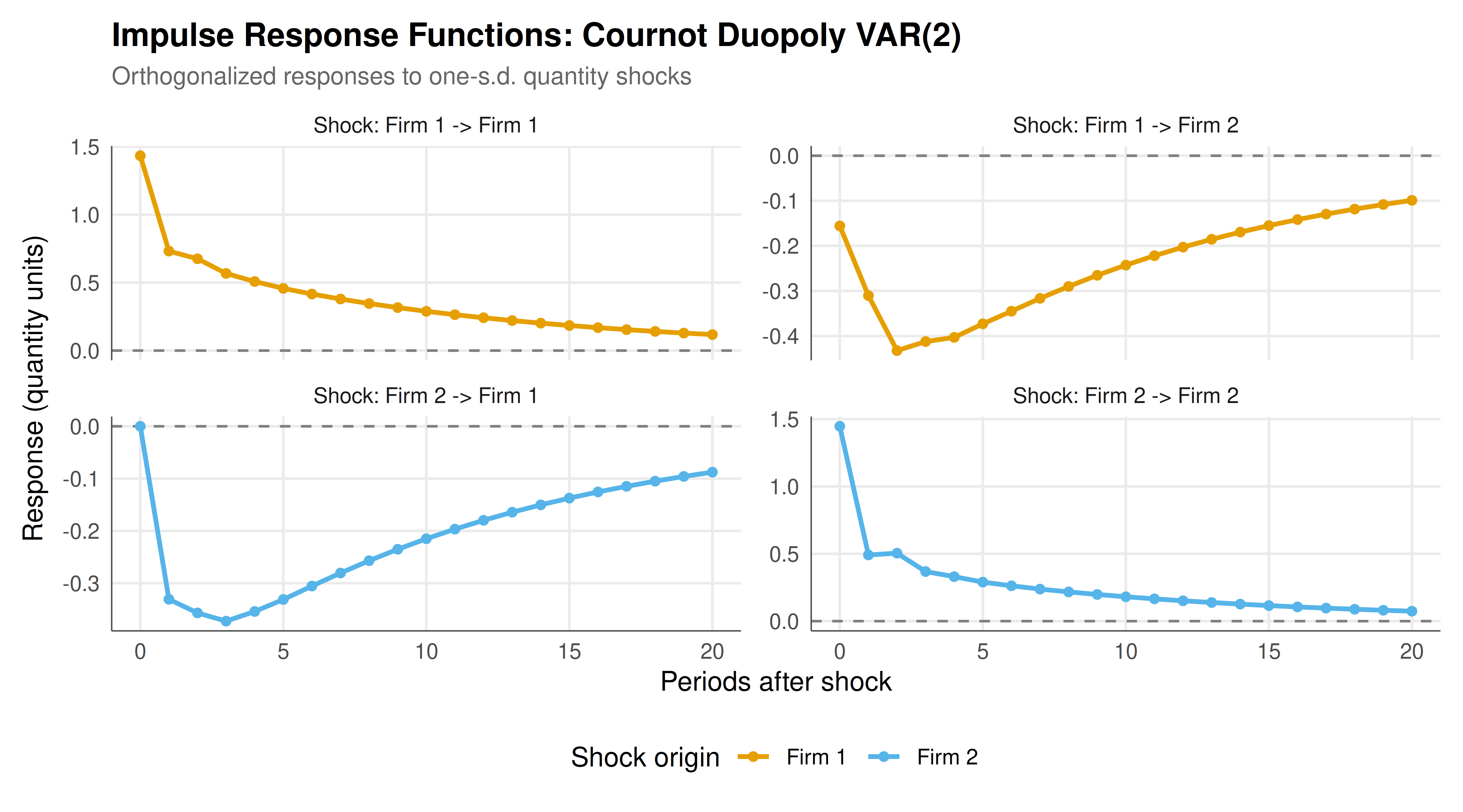
We compute orthogonalized impulse response functions over 20 periods using the Cholesky decomposition of the residual covariance matrix and plot all four response combinations.

# --- Compute IRFs via recursive MA representation ---
A1_hat <- matrix(c(B_hat["q1_lag1", "q1_eq"], B_hat["q1_lag1", "q2_eq"],
                    B_hat["q2_lag1", "q1_eq"], B_hat["q2_lag1", "q2_eq"]),
                  nrow = 2, byrow = TRUE)
A2_hat <- matrix(c(B_hat["q1_lag2", "q1_eq"], B_hat["q1_lag2", "q2_eq"],
                    B_hat["q2_lag2", "q1_eq"], B_hat["q2_lag2", "q2_eq"]),
                  nrow = 2, byrow = TRUE)

# Cholesky decomposition for orthogonalized IRFs
P <- t(chol(Sigma_hat))

H <- 20  # IRF horizon
Phi <- array(0, dim = c(2, 2, H + 1))
Phi[, , 1] <- diag(2)

for (s in 2:(H + 1)) {
  if (s - 1 >= 1) Phi[, , s] <- Phi[, , s] + Phi[, , s - 1] %*% A1_hat

  if (s - 2 >= 1) Phi[, , s] <- Phi[, , s] + Phi[, , s - 2] %*% A2_hat
}

# Orthogonalized IRFs: Theta_s = Phi_s %*% P
Theta <- array(0, dim = c(2, 2, H + 1))
for (s in 1:(H + 1)) {
  Theta[, , s] <- Phi[, , s] %*% P
}

# Build data frame for plotting
irf_df <- expand.grid(horizon = 0:H, response = c("Firm 1", "Firm 2"),
                       impulse = c("Firm 1", "Firm 2"))
irf_df$value <- NA
for (i in 1:2) {
  for (j in 1:2) {
    idx <- irf_df$response == paste("Firm", i) & irf_df$impulse == paste("Firm", j)
    irf_df$value[idx] <- Theta[i, j, ]
  }
}
irf_df$panel <- paste("Shock:", irf_df$impulse, "->", irf_df$response)

p_irf <- ggplot(irf_df, aes(x = horizon, y = value, color = impulse)) +
  geom_hline(yintercept = 0, linetype = "dashed", color = "grey50") +
  geom_line(linewidth = 1) +
  geom_point(size = 1.5) +
  facet_wrap(~ panel, scales = "free_y", ncol = 2) +
  scale_color_manual(values = okabe_ito[1:2]) +
  labs(title = "Impulse Response Functions: Cournot Duopoly VAR(2)",
       subtitle = "Orthogonalized responses to one-s.d. quantity shocks",
       x = "Periods after shock", y = "Response (quantity units)",
       color = "Shock origin") +
  theme_publication()

p_irf

Figure 1: Figure 1. Orthogonalized impulse response functions for a Cournot duopoly VAR(2) model. Each panel shows the dynamic response of one firm’s output to a one-standard-deviation shock in the other firm’s (or its own) quantity innovation. Negative cross-responses confirm strategic substitutability. Data: simulated (CC BY-SA 4.0).

Interactive figure

The interactive version allows hovering over each point to see the exact IRF value at each horizon, facilitating detailed inspection of strategic adjustment dynamics.

irf_df$text <- paste0("Horizon: ", irf_df$horizon,
                       "\nResponse: ", round(irf_df$value, 3),
                       "\nShock: ", irf_df$impulse,
                       " -> ", irf_df$response)

p_irf_int <- ggplot(irf_df, aes(x = horizon, y = value, color = impulse, text = text)) +
  geom_hline(yintercept = 0, linetype = "dashed", color = "grey50") +
  geom_line(linewidth = 0.8) +
  geom_point(size = 1.5) +
  facet_wrap(~ panel, scales = "free_y", ncol = 2) +
  scale_color_manual(values = okabe_ito[1:2]) +
  labs(title = "IRFs: Cournot Duopoly VAR(2)",
       x = "Periods after shock", y = "Response",
       color = "Shock origin") +
  theme_publication()

ggplotly(p_irf_int, tooltip = "text") |>
  config(displaylogo = FALSE)

Figure 2

Interpretation

The VAR(2) estimation results reveal a rich picture of dynamic strategic interaction between the two duopolists. The coefficient estimates on the rival’s lagged quantities are negative, confirming the strategic substitutability that is characteristic of Cournot competition: when one firm increased output last period, the other responds by reducing its own output this period. This is entirely consistent with the theoretical prediction from best-response functions in the static Cournot model, but the VAR captures the quantitative magnitude and temporal structure of these reactions in a way that static analysis cannot.

The own-lag coefficients are positive and less than one, indicating that each firm’s output is persistent but stationary. Firm 1’s output depends on roughly half of its own previous quantity plus a small positive effect from two periods ago. This persistence means that strategic adjustments play out gradually over multiple periods rather than snapping instantly to the Nash equilibrium. The dynamic path toward equilibrium is a key feature that distinguishes actual market competition from the timeless equilibrium concept in textbook game theory.

The Granger causality tests provide formal statistical evidence for the strategic interdependence between the two firms. Both tests reject the null hypothesis that the rival’s lagged quantities have no predictive power, confirming bidirectional Granger causality. This means that knowing firm 2’s past output helps predict firm 1’s current output, even after accounting for firm 1’s own history, and vice versa. In the context of strategic interaction, Granger causality is a natural empirical counterpart to the game-theoretic concept of strategic interdependence: each firm’s payoff, and therefore its optimal action, depends on what the other firm does.

The impulse response functions tell the most compelling story. When firm 1 experiences a positive quantity shock (an unexpected increase in output), firm 2 responds by reducing its own output in the following periods. The cross-firm IRF is negative, reflecting the substitution effect, and it decays back to zero over approximately 8 to 12 periods. The own-response IRF starts at the shock size and also decays back to zero, but through a different path that may exhibit mild oscillation as the two firms engage in a back-and-forth adjustment process. This oscillatory pattern is characteristic of dynamic strategic interaction where each firm is reacting to the other’s most recent move, creating a feedback loop that takes several rounds to settle.

The residual covariance matrix reveals the contemporaneous correlation between the two firms’ innovations. A negative correlation would suggest that within-period shocks tend to push the firms in opposite directions, which would be consistent with short-run competitive displacement. A positive correlation might indicate common demand or cost shocks affecting both firms simultaneously. The Cholesky decomposition used for orthogonalized IRFs imposes a causal ordering (firm 1’s shocks can affect firm 2 contemporaneously but not vice versa), which is an identifying assumption. In practice, the choice of ordering matters when the residual correlation is large, and researchers often report results under both orderings as a robustness check.

From a game-theoretic perspective, the VAR framework bridges the gap between the elegant simplicity of static Nash equilibrium and the messy reality of dynamic competition. The Nash equilibrium of the static Cournot game corresponds to the long-run steady state of the VAR (where both firms’ quantities have converged to their unconditional means and shocks have dissipated). But the VAR reveals the adjustment dynamics around that equilibrium, the speed of convergence, the role of rival feedback, and the volatility contributed by each firm’s shocks. For applied researchers studying real markets (airlines, telecommunications, retail), the VAR approach provides actionable insights about the timing and magnitude of competitive responses that static game theory simply cannot deliver.

One important limitation is that VAR models are reduced-form: they capture statistical regularities in the data but do not impose or test the structural optimization that underlies game-theoretic models. The estimated coefficients are functions of the underlying payoff parameters, demand elasticities, and cost structures, but the VAR itself does not identify these primitives. Structural VAR (SVAR) approaches can address this by imposing theory-based restrictions on the contemporaneous relationships between variables, and the growing literature on dynamic games provides complementary structural estimation techniques.

Extensions & related tutorials

The VAR framework for strategic interaction connects to several other methods and models covered elsewhere on this site:

• Cournot duopoly static equilibrium – the static benchmark that the VAR dynamics orbit around
• Repeated games and folk theorem – the theoretical foundation for sustained dynamic interaction
• Bayesian VAR for game-theoretic inference – shrinkage priors improve small-sample VAR estimation
• Structural estimation of dynamic games – recovering payoff primitives from observed play sequences
• Network games and spatial interaction – extending pairwise VAR to multi-player network settings

References