

Prerequisite. This vignette assumes the API from Getting Started with tesseractR. If you’d rather just play, the four-part tutorial starts at The rules of 4D tic-tac-toe.
tesseractR is also a study tool: a single
evaluation core (tsr_evaluate() /
tsr_win_prob() / tsr_rate_moves()) powers
self-play simulation, per-ply game analysis, and aggregate behavioral
profiles. Everything below routes through that core — no parallel
scoring logic.
A single self-play game
g <- tsr_play_game("greedy", "random", seed = 7L)
g
#>
#> ── <tsr_game> ──
#>
#> X policy: greedy
#> O policy: random
#> Result: X wins after 19 moves
The tsr_game object records the move sequence, who moved
on each ply, the final board, the outcome, and the policy labels.
Replaying the moves on a fresh board reproduces final_board
exactly.
tsr_plot(g$final_board)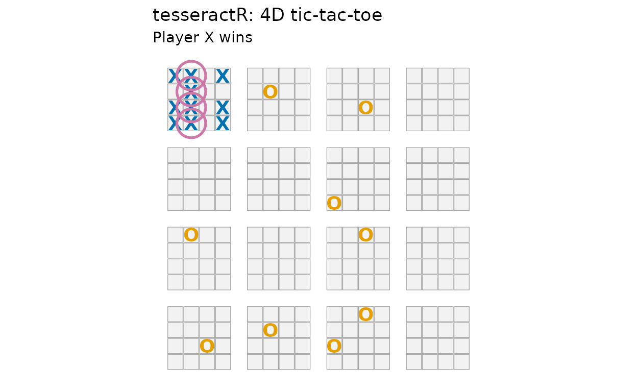
Per-ply analysis
tsr_analyze_game() walks the game and for each ply
records: win-probability before/after, the move’s delta,
the best alternative, regret, and flags for missed wins, missed blocks,
and turning points (abs(delta) >= 0.15).
analysis <- tsr_analyze_game(g)
tail(analysis, 6)
#> # A tibble: 6 × 17
#>     ply player  cell     i     j     k     l win_prob_before win_prob_after
#>   <int>  <int> <int> <int> <int> <int> <int>           <dbl>          <dbl>
#> 1    14      2    22     1     1     1     0         0.0227         0.0258
#> 2    15      1    16     3     3     0     0         0.974          0.991
#> 3    16      2   233     0     2     2     3         0.00915        0.00964
#> 4    17      1    14     1     3     0     0         0.990          0.998
#> 5    18      2   130     1     0     0     2         0.00190        0.00200
#> 6    19      1     6     1     1     0     0         0.998          1
#> # ℹ 8 more variables: delta <dbl>, best_cell <int>, best_delta <dbl>,
#> #   regret <dbl>, is_best <lgl>, missed_win <lgl>, missed_block <lgl>,
#> #   is_turning_point <lgl>
tsr_plot_winprob(analysis)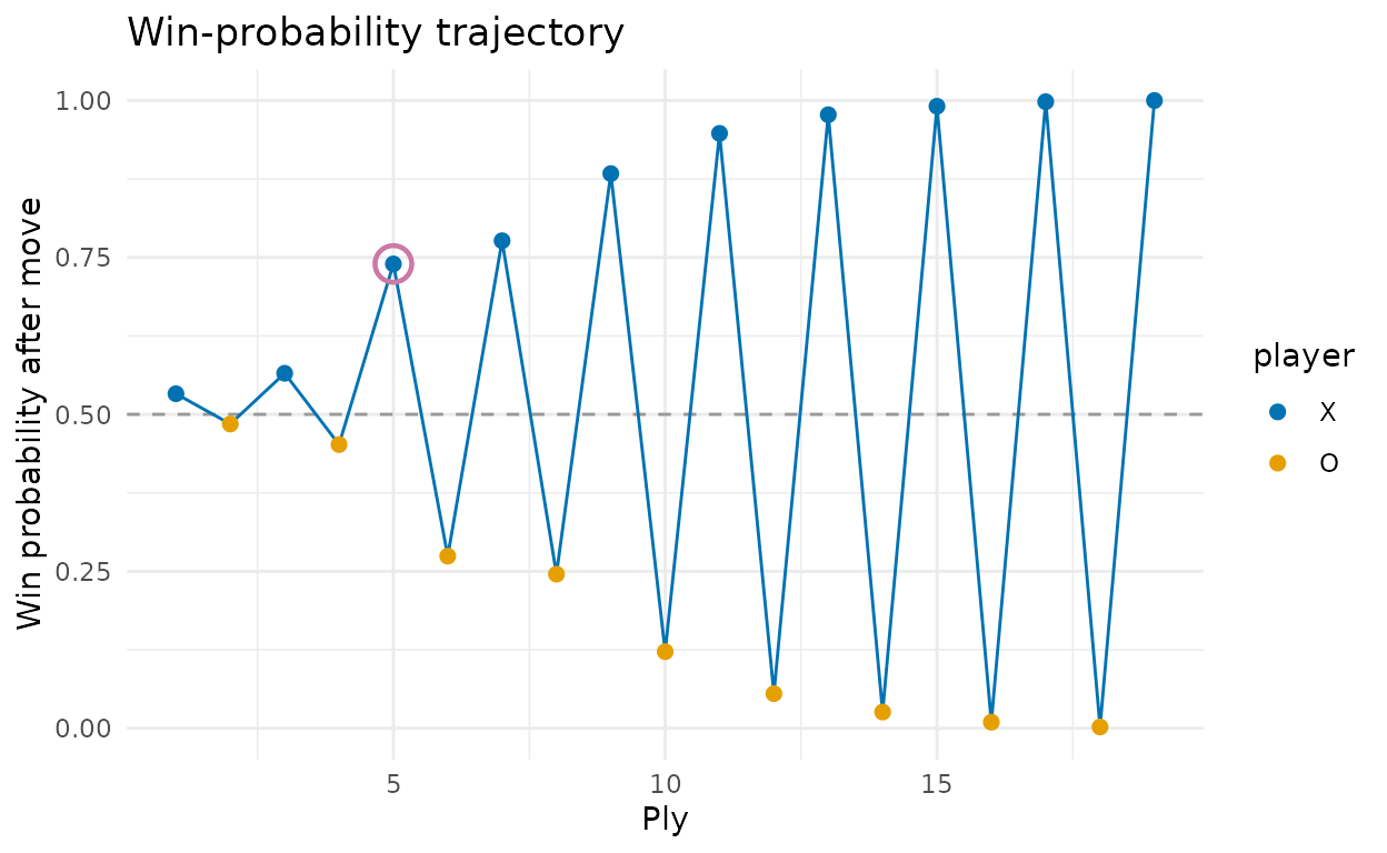
tsr_turning_points(analysis)
#> # A tibble: 1 × 17
#>     ply player  cell     i     j     k     l win_prob_before win_prob_after
#>   <int>  <int> <int> <int> <int> <int> <int>           <dbl>          <dbl>
#> 1     5      1     2     1     0     0     0           0.548          0.740
#> # ℹ 8 more variables: delta <dbl>, best_cell <int>, best_delta <dbl>,
#> #   regret <dbl>, is_best <lgl>, missed_win <lgl>, missed_block <lgl>,
#> #   is_turning_point <lgl>
tsr_game_summary(g)
#> # A tibble: 1 × 10
#>   winner n_moves n_missed_wins_x n_missed_wins_o n_missed_blocks_x
#>    <int>   <int>           <int>           <int>             <int>
#> 1      1      19               6               0                 0
#> # ℹ 5 more variables: n_missed_blocks_o <int>, mean_regret_x <dbl>,
#> #   mean_regret_o <dbl>, n_turning_points <int>, decisiveness <dbl>
Self-play in bulk
tsr_simulate() runs many games and returns a tibble with
the first-move position broken into its four coordinates — the substrate
for opening statistics.
Performance. Pure-R self-play is throughput-bounded; the heavy hot paths (
tsr_evaluate, legal-move generation) are flagged for future Rcpp replacement. Meaningful opening statistics need thousands of games; the example below is deliberately tiny so the vignette builds in seconds.
sim <- tsr_simulate("random", "random", n_games = 12L,
                    seed = 1L, verbose = FALSE)
sim
#> # A tibble: 12 × 10
#>    game_id policy_x policy_o winner n_moves first_move first_move_i first_move_j
#>      <int> <chr>    <chr>     <int>   <int>      <int>        <int>        <int>
#>  1       1 random   random        2     100        249            0            2
#>  2       2 random   random        1      81        107            2            2
#>  3       3 random   random        2      98        174            1            3
#>  4       4 random   random        1      55         31            2            3
#>  5       5 random   random        1     141        103            2            1
#>  6       6 random   random        2      82         47            2            3
#>  7       7 random   random        2      44         87            2            1
#>  8       8 random   random        1      85        115            2            0
#>  9       9 random   random        1      85        112            3            3
#> 10      10 random   random        1     129        211            2            0
#> 11      11 random   random        1      45        244            3            0
#> 12      12 random   random        1     119        138            1            2
#> # ℹ 2 more variables: first_move_k <int>, first_move_l <int>
opening <- tsr_opening_stats(sim, by = "first_move")
head(opening, 8)
#> # A tibble: 8 × 7
#>   first_move n_games win_rate_x win_rate_o draw_rate ci_lo ci_hi
#>        <int>   <int>      <dbl>      <dbl>     <dbl> <dbl> <dbl>
#> 1         31       1          1          0         0 0.207 1
#> 2         47       1          0          1         0 0     0.793
#> 3         87       1          0          1         0 0     0.793
#> 4        103       1          1          0         0 0.207 1
#> 5        107       1          1          0         0 0.207 1
#> 6        112       1          1          0         0 0.207 1
#> 7        115       1          1          0         0 0.207 1
#> 8        138       1          1          0         0 0.207 1
The opening-statistics tibble carries a Wilson 95% confidence
interval on win_rate_x — small n_games means
wide intervals. A few hundred games per opening would be needed to draw
real conclusions; this vignette uses a deliberately tiny sample so it
builds in seconds.
Policy behavioral profile
tsr_behavior_profile() aggregates per-ply analyses
across many games into a single behavioral signature for one side. Use
tsr_compare_profiles() to stack profiles side by side.
games_r <- lapply(1:3, function(s) tsr_play_game("random", "random", seed = s))
games_g <- lapply(1:3, function(s) tsr_play_game("greedy", "random", seed = s))
p_random <- tsr_behavior_profile(games_r, side = 1L, label = "X random")
p_greedy <- tsr_behavior_profile(games_g, side = 1L, label = "X greedy")
tsr_compare_profiles(p_random, p_greedy)
#> # A tibble: 2 × 11
#>   label     side n_games n_moves_total accuracy mean_regret blunder_rate
#>   <chr>    <int>   <int>         <int>    <dbl>       <dbl>        <dbl>
#> 1 X random     1       3           136    0          0.387        0.860
#> 2 X greedy     1       3            68    0.132      0.0206       0.0882
#> # ℹ 4 more variables: win_conversion <dbl>, defense_rate <dbl>,
#> #   aggression <dbl>, mean_decisiveness <dbl>
Read the rows side-by-side: accuracy is the share of
plies that matched the engine’s top move; blunder_rate is
the share with regret above the documented threshold;
aggression is the share of moves that opened a new
3-in-line threat for the side.
Where this all meets the app
The same tsr_win_prob() powers the app’s live
win-probability gauge, the same tsr_rate_moves() powers the
per-cell rating overlay, and the same tsr_analyze_game()
powers the post-game analysis tab — so a number you see in the UI
matches exactly what these functions produce from the console.