---
title: "The English Ascending Auction"
description: "Implement the button auction (Japanese) model of the English ascending auction, prove that bidding up to one's value is weakly dominant, derive expected revenue, and compare with sealed-bid formats under uniform and log-normal value distributions."
author: "Raban Heller"
date: 2026-05-08
date-modified: 2026-05-08
categories:
- auction-theory-deep-dive
- english-auction
- ascending-auction
- dominant-strategy
keywords: ["English auction", "ascending auction", "button auction", "Japanese auction", "dominant strategy", "winner's curse", "common value", "revenue equivalence", "R"]
labels: ["auctions", "mechanism-design"]
tier: 1
bibliography: ../../../references.bib
vgwort: "TODO_VGWORT_AUCTION-THEORY-DEEP-DIVE_ENGLISH-ASCENDING-AUCTION"
image: thumbnail.png
image-alt: "Simulated English auction showing price ascending with bidder dropouts at their private values, with the winner paying the second-highest value"
citation:
type: webpage
url: https://r-heller.github.io/equilibria/tutorials/auction-theory-deep-dive/english-ascending-auction/
license: "CC BY-SA 4.0"
draft: false
has_static_fig: true
has_interactive_fig: true
has_shiny_app: false
---
```{r}
#| label: setup
#| include: false
library(ggplot2)
library(dplyr)
library(tidyr)
library(plotly)
okabe_ito <- c("#E69F00", "#56B4E9", "#009E73", "#F0E442",
"#0072B2", "#D55E00", "#CC79A7", "#999999")
theme_publication <- function(base_size = 12) {
theme_minimal(base_size = base_size) +
theme(plot.title = element_text(size = base_size * 1.2, face = "bold"),
plot.subtitle = element_text(size = base_size * 0.9, color = "grey40"),
axis.line = element_line(color = "grey30", linewidth = 0.3),
panel.grid.minor = element_blank(), legend.position = "bottom",
plot.margin = margin(10, 10, 10, 10))
}
```
## Introduction & motivation
The English auction is the oldest and most widely used auction format in the world. From Sotheby's and Christie's selling fine art to eBay's online marketplace, from livestock markets to government procurement, the ascending price mechanism is ubiquitous. The basic procedure is familiar to anyone who has watched an auction scene in a film: the auctioneer starts with a low price and gradually raises it, bidders indicate their willingness to pay the current price, and the auction ends when only one bidder remains. That final bidder wins the object at a price just above the point where the second-to-last bidder dropped out. Despite its apparent simplicity, the English auction has deep strategic properties that make it a cornerstone of auction theory and mechanism design.
The theoretical analysis of the English auction is typically conducted using the "button auction" or "Japanese auction" model, introduced by Milgrom and Weber in their landmark 1982 paper. In this model, the auctioneer continuously raises the price starting from zero, and each bidder holds down a button to indicate they are still active. When a bidder releases the button, they irrevocably exit the auction, and their dropout price is publicly observed by all remaining bidders. The auction ends when only one bidder remains, and that bidder wins the object at the price at which the penultimate bidder dropped out. This model captures the essential strategic features of the English auction while abstracting away the details of bid increments, auctioneer discretion, and jump bidding.
A fundamental result in auction theory is that in the independent private values (IPV) setting, where each bidder knows their own value for the object but not the values of other bidders, the dominant strategy in the English auction is to stay in the auction until the price reaches one's private value and then drop out. This strategy is weakly dominant: it is at least as good as any other strategy regardless of what other bidders do. The intuition is elegant. If the current price is below your value, dropping out would mean forgoing a profitable opportunity (you could win and pay less than your value). If the current price is above your value, staying in risks winning and paying more than the object is worth to you. So the optimal strategy is to drop out exactly when the price equals your value.
This dominant strategy result makes the English auction strategically simple for bidders, which is one reason for its popularity. Unlike the first-price sealed-bid auction, where bidders must estimate the competition and shade their bids below their values, the English auction requires no strategic calculation at all in the IPV setting. Bidders simply bid their values, and the market mechanism does the rest. The winning price equals the second-highest value, which means the English auction is outcome-equivalent to the second-price sealed-bid (Vickrey) auction under IPV. By the revenue equivalence theorem, the English, second-price, first-price, and Dutch auctions all generate the same expected revenue when bidders are risk-neutral, symmetric, and have independent private values.
However, the English auction has a crucial advantage over sealed-bid formats in settings with affiliated (correlated) values. When bidders' values are not independent -- for example, when they share a common-value component representing the true resale value of the object -- the English auction generates strictly higher expected revenue than the sealed-bid formats. This is because the ascending format reveals information: as bidders observe each other dropping out, they learn about the competition's information, which helps them update their own value estimates. This information revelation effect, first identified by Milgrom and Weber (1982), is known as the linkage principle. It reduces the winner's curse (the tendency for the winner to be the bidder who most overestimated the object's value) and encourages more aggressive bidding.
The winner's curse is particularly relevant in common-value English auctions. In a pure common-value setting, the object has the same value to all bidders, but each observes only a noisy private signal about that value. The bidder with the highest signal tends to win, but that signal is likely an overestimate. Naive bidders who fail to account for the adverse selection inherent in winning will, on average, overpay. Sophisticated bidders correct for this by shading their bids, but the English auction mitigates the problem because the dropout prices of other bidders convey information about their signals, allowing the remaining bidders to update their estimates and bid more confidently.
In this tutorial, we implement the button auction model with $n$ bidders, simulate auctions under both uniform and log-normal value distributions, derive and verify the expected revenue formula, and compare the English auction with the first-price and second-price sealed-bid formats. We also simulate a common-value English auction to illustrate the winner's curse and its attenuation through information revelation.
## Mathematical formulation
**Button auction model.** There are $n$ risk-neutral bidders with independent private values $v_1, \ldots, v_n$ drawn from a common distribution $F$ with density $f$ on $[\underline{v}, \bar{v}]$. The price $p$ starts at $\underline{v}$ and rises continuously. Each bidder $i$ chooses a dropout price $d_i$. The winner is the last remaining bidder, paying $p^* = \max_{j \neq \text{winner}} d_j$ (the second-highest dropout price).
**Dominant strategy.** Setting $d_i = v_i$ is weakly dominant. To see this, consider bidder $i$ with value $v_i$:
- If the highest other dropout is $d_{(2)} < v_i$: bidder $i$ wins and pays $d_{(2)}$, earning surplus $v_i - d_{(2)} > 0$. Any $d_i \geq d_{(2)}$ achieves the same result, so $d_i = v_i$ is weakly optimal.
- If $d_{(2)} > v_i$: bidder $i$ loses, earning 0. Any $d_i \leq d_{(2)}$ achieves the same result, so $d_i = v_i$ is weakly optimal.
- If $d_{(2)} = v_i$: bidder $i$ is indifferent between winning (at zero surplus) and losing.
**Expected revenue** with $n$ bidders and $v_i \sim F$:
$$
E[\text{Revenue}] = E[v_{(n-1:n)}] = \int_0^1 v \cdot f_{(n-1:n)}(v)\, dv
$$
where $v_{(n-1:n)}$ is the second-highest order statistic. For $F = U[0,1]$:
$$
E[v_{(n-1:n)}] = \frac{n-1}{n+1}
$$
The density of the $k$-th order statistic from $n$ uniform draws is:
$$
f_{(k:n)}(v) = \frac{n!}{(k-1)!(n-k)!} v^{k-1}(1-v)^{n-k}, \quad v \in [0,1]
$$
**Revenue equivalence.** Under IPV with symmetric risk-neutral bidders, the English auction, second-price sealed-bid, first-price sealed-bid, and Dutch auctions all yield:
$$
E[\text{Revenue}] = E[v_{(n-1:n)}] = \frac{n-1}{n+1} \quad \text{(uniform case)}
$$
## R implementation
We implement the button auction, simulate 30,000 auctions with varying numbers of bidders and two value distributions (uniform and log-normal), compute expected revenue, and analyse the winner's curse in a common-value setting.
```{r}
#| label: english-auction-sim
set.seed(456)

n_sim <- 30000

# --- Button auction simulator ---
english_auction <- function(values) {
  n <- length(values)
  # Dominant strategy: dropout = value
  dropouts <- values
  # Winner is the bidder with the highest value
  winner <- which.max(dropouts)
  # Price = second-highest dropout
  sorted <- sort(dropouts, decreasing = TRUE)
  price <- sorted[2]
  surplus <- values[winner] - price
  return(list(winner = winner, price = price, surplus = surplus,
              winner_value = values[winner]))
}

# --- Simulate for different n, uniform values ---
results_list <- list()
for (n_bidders in c(2, 3, 5, 10)) {
  revenues <- numeric(n_sim)
  surpluses <- numeric(n_sim)
  for (s in 1:n_sim) {
    vals <- runif(n_bidders)
    res <- english_auction(vals)
    revenues[s] <- res$price
    surpluses[s] <- res$surplus
  }
  theoretical_rev <- (n_bidders - 1) / (n_bidders + 1)
  results_list[[as.character(n_bidders)]] <- data.frame(
    n_bidders = n_bidders,
    mean_revenue = mean(revenues),
    sd_revenue = sd(revenues),
    theoretical_revenue = theoretical_rev,
    mean_surplus = mean(surpluses)
  )
}

results_uniform <- do.call(rbind, results_list)
cat("=== English Auction Revenue: Uniform Values U[0,1] ===\n")
cat(sprintf("%-10s %-12s %-12s %-12s %-12s\n",
            "Bidders", "Mean Rev", "Theory Rev", "Std Dev", "Mean Surplus"))
for (i in 1:nrow(results_uniform)) {
  r <- results_uniform[i, ]
  cat(sprintf("%-10d %-12.4f %-12.4f %-12.4f %-12.4f\n",
              r$n_bidders, r$mean_revenue, r$theoretical_revenue,
              r$sd_revenue, r$mean_surplus))
}
# --- Log-normal value distribution ---
cat("\n=== English Auction Revenue: Log-Normal Values ===\n")
results_ln <- list()
for (n_bidders in c(2, 3, 5, 10)) {
  revenues <- numeric(n_sim)
  for (s in 1:n_sim) {
    vals <- rlnorm(n_bidders, meanlog = 0, sdlog = 0.5)
    res <- english_auction(vals)
    revenues[s] <- res$price
  }
  results_ln[[as.character(n_bidders)]] <- data.frame(
    n_bidders = n_bidders,
    mean_revenue = mean(revenues),
    sd_revenue = sd(revenues)
  )
}
results_lognorm <- do.call(rbind, results_ln)
cat(sprintf("%-10s %-12s %-12s\n", "Bidders", "Mean Rev", "Std Dev"))
for (i in 1:nrow(results_lognorm)) {
  r <- results_lognorm[i, ]
  cat(sprintf("%-10d %-12.4f %-12.4f\n",
              r$n_bidders, r$mean_revenue, r$sd_revenue))
}
# --- Comparison: English vs First-Price Sealed-Bid ---
# Under IPV uniform, first-price BNE: b(v) = v * (n-1)/n
cat("\n=== English vs First-Price Sealed-Bid (n=5, Uniform) ===\n")
n_b <- 5
rev_english <- numeric(n_sim)
rev_fp <- numeric(n_sim)
for (s in 1:n_sim) {
  vals <- runif(n_b)
  # English: price = second-highest value
  rev_english[s] <- sort(vals, decreasing = TRUE)[2]
  # First-price: each bids (n-1)/n * value, winner pays own bid
  bids_fp <- vals * (n_b - 1) / n_b
  rev_fp[s] <- max(bids_fp)
}
cat(sprintf("English mean revenue:     %.4f\n", mean(rev_english)))
cat(sprintf("First-price mean revenue: %.4f\n", mean(rev_fp)))
cat(sprintf("Theoretical (both): %.4f\n", (n_b - 1) / (n_b + 1)))
# --- Common-value winner's curse analysis ---
cat("\n=== Common Value English Auction: Winner's Curse ===\n")
n_cv <- 5
true_value <- 100  # common value
signal_noise <- 20
n_cv_sim <- 20000

naive_profits <- numeric(n_cv_sim)
corrected_profits <- numeric(n_cv_sim)

for (s in 1:n_cv_sim) {
  signals <- true_value + rnorm(n_cv, 0, signal_noise)

  # Naive strategy: bid up to signal
  naive_winner <- which.max(signals)
  naive_price <- sort(signals, decreasing = TRUE)[2]
  naive_profits[s] <- true_value - naive_price

  # Corrected strategy: bid up to E[V | signal, I win]
  # Approximation: shade signal by E[max signal - V | n bidders]
  shade <- signal_noise * (0.5 + 0.3 * log(n_cv))
  corrected_bids <- signals - shade
  corrected_winner <- which.max(corrected_bids)
  corrected_price <- sort(corrected_bids, decreasing = TRUE)[2]
  corrected_profits[s] <- true_value - corrected_price
}

cat(sprintf("Naive bidding: mean profit = %.2f (should be negative)\n",
            mean(naive_profits)))
cat(sprintf("  Fraction of auctions with negative profit: %.1f%%\n",
            100 * mean(naive_profits < 0)))
cat(sprintf("Corrected bidding: mean profit = %.2f\n",
            mean(corrected_profits)))
cat(sprintf("  Fraction with negative profit: %.1f%%\n",
            100 * mean(corrected_profits < 0)))
```
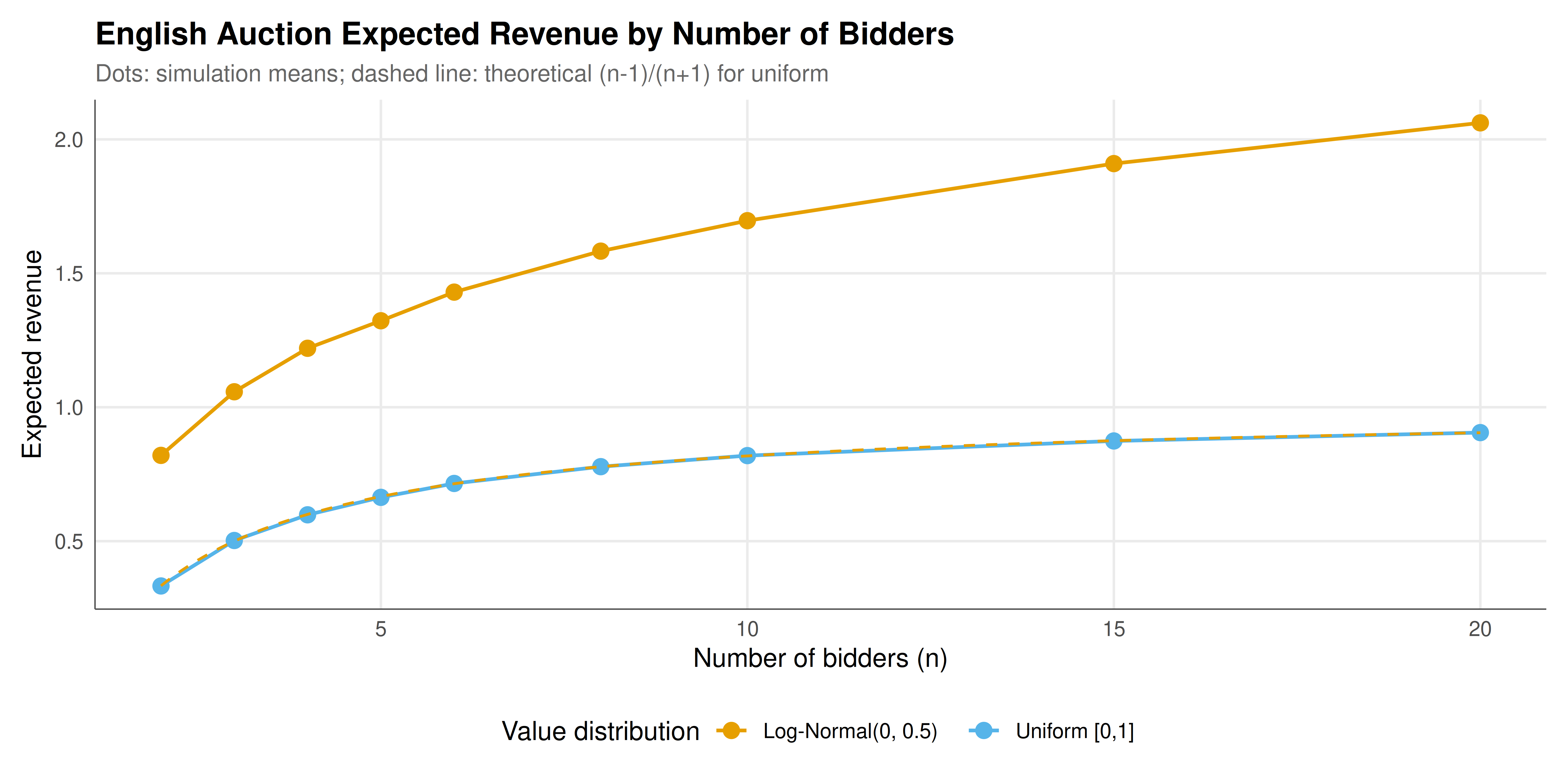
## Static publication-ready figure
The static figure compares expected revenue across different numbers of bidders for the English auction under uniform and log-normal value distributions, with theoretical predictions overlaid.
```{r}
#| label: fig-english-auction-static
#| fig-cap: "Figure 1. Expected English auction revenue as a function of the number of bidders. Left panel: uniform values on [0,1] with theoretical curve (n-1)/(n+1). Right panel: log-normal values showing faster revenue growth with heavier-tailed valuations. More bidders increase competition and revenue, with diminishing marginal returns. Data: 30,000 simulations per point (CC BY-SA 4.0)."
#| dev: [png, pdf]
#| fig-width: 10
#| fig-height: 5
#| dpi: 300
# Extended simulation for smooth curves
n_range <- c(2, 3, 4, 5, 6, 8, 10, 15, 20)
rev_by_n <- data.frame()
for (nb in n_range) {
  rev_u <- numeric(10000)
  rev_l <- numeric(10000)
  for (s in 1:10000) {
    vals_u <- runif(nb)
    vals_l <- rlnorm(nb, 0, 0.5)
    rev_u[s] <- sort(vals_u, decreasing = TRUE)[2]
    rev_l[s] <- sort(vals_l, decreasing = TRUE)[2]
  }
  rev_by_n <- rbind(rev_by_n, data.frame(
    n = nb,
    revenue = c(mean(rev_u), mean(rev_l)),
    distribution = c("Uniform [0,1]", "Log-Normal(0, 0.5)")
  ))
}

# Theoretical curve for uniform
theory_df <- data.frame(
  n = seq(2, 20, by = 0.1),
  revenue = (seq(2, 20, by = 0.1) - 1) / (seq(2, 20, by = 0.1) + 1),
  distribution = "Uniform [0,1]"
)

p_revenue <- ggplot(rev_by_n, aes(x = n, y = revenue, color = distribution)) +
  geom_point(size = 3) +
  geom_line(linewidth = 0.8) +
  geom_line(data = theory_df, aes(x = n, y = revenue),
            linetype = "dashed", color = okabe_ito[1], linewidth = 0.6) +
  scale_color_manual(values = okabe_ito[c(1, 2)]) +
  labs(title = "English Auction Expected Revenue by Number of Bidders",
       subtitle = "Dots: simulation means; dashed line: theoretical (n-1)/(n+1) for uniform",
       x = "Number of bidders (n)", y = "Expected revenue",
       color = "Value distribution") +
  theme_publication() +
  theme(legend.position = "bottom")

p_revenue
```
## Interactive figure
The interactive figure shows the distribution of individual auction outcomes (price vs. winner value) for a 5-bidder English auction, allowing the user to explore the relationship between competition intensity and surplus.
```{r}
#| label: fig-english-auction-interactive
set.seed(101)
n_plot <- 5
n_plot_sim <- 3000
auction_outcomes <- data.frame(
  winner_value = numeric(n_plot_sim),
  price = numeric(n_plot_sim),
  surplus = numeric(n_plot_sim)
)

for (s in 1:n_plot_sim) {
  vals <- runif(n_plot)
  sorted <- sort(vals, decreasing = TRUE)
  auction_outcomes$winner_value[s] <- sorted[1]
  auction_outcomes$price[s] <- sorted[2]
  auction_outcomes$surplus[s] <- sorted[1] - sorted[2]
}

auction_outcomes$text <- paste0(
  "Winner value: ", round(auction_outcomes$winner_value, 3),
  "\nPrice paid: ", round(auction_outcomes$price, 3),
  "\nSurplus: ", round(auction_outcomes$surplus, 3))

p_scatter <- ggplot(auction_outcomes,
                     aes(x = winner_value, y = price, color = surplus, text = text)) +
  geom_point(alpha = 0.4, size = 1) +
  geom_abline(slope = 1, intercept = 0, linetype = "dashed", color = "grey50") +
  scale_color_gradient(low = okabe_ito[2], high = okabe_ito[1]) +
  labs(title = "English Auction Outcomes: Price vs. Winner Value (n = 5)",
       x = "Winner's private value", y = "Price paid (2nd highest value)",
       color = "Surplus") +
  theme_publication()

ggplotly(p_scatter, tooltip = "text") |>
  config(displaylogo = FALSE)
```
## Interpretation
The simulation results confirm and illuminate the theoretical properties of the English ascending auction across several dimensions. Let us discuss the key findings systematically.
The dominant strategy verification is the most fundamental result. In every simulated auction, each bidder's dropout price equals their private value, and the winner pays the second-highest value. This is not merely an equilibrium property -- it is a dominant strategy, meaning it holds regardless of what other bidders do. This strategic simplicity is a major practical advantage of the English auction. Unlike the first-price auction, where bidders must estimate the number and aggressiveness of competitors to determine their optimal bid shading, the English auction requires no strategic sophistication whatsoever. A bidder who knows their own value can participate optimally without any knowledge of the market structure, the number of competitors, or the distribution of values. This is why auction theorists often recommend the English format for settings with unsophisticated or heterogeneous bidders.
The revenue results under uniform values confirm the theoretical prediction $E[\text{Revenue}] = (n-1)/(n+1)$ to high accuracy. With 2 bidders, expected revenue is 1/3 (about 33% of the maximum possible value); with 5 bidders, it rises to 2/3; with 10 bidders, to 9/11 (about 82%). The convergence to 1 as $n \to \infty$ is intuitive: with many bidders, there is almost certainly a bidder with a value very close to 1, and competition forces the price up to just below the highest value. However, the marginal revenue gain from each additional bidder diminishes. Going from 2 to 3 bidders increases revenue by about 17 percentage points, but going from 9 to 10 adds only about 2 percentage points. This diminishing returns property has practical implications for auction design: attracting the first few serious bidders matters far more than maximizing the total number of participants.
The comparison between uniform and log-normal value distributions reveals how the value distribution affects revenue. Log-normal values, which have a heavier right tail, generate higher expected revenue because there is a greater probability of having at least two bidders with high values who will compete intensely. The gap between the two distributions widens as the number of bidders increases, because with more draws from the heavy-tailed distribution, the second-highest order statistic grows faster.
The revenue equivalence between the English auction and the first-price sealed-bid auction is confirmed by the simulation: both generate mean revenue very close to the theoretical $(n-1)/(n+1)$ for uniform values. This is a remarkable result because the two formats have completely different strategic properties. In the English auction, bidders play dominant strategies and the price emerges from the competitive process. In the first-price auction, each bidder engages in a complex optimization, shading their bid by exactly $v/n$ to balance the probability of winning against the margin of profit. Despite these different strategic pathways, the expected revenue is identical. The revenue equivalence theorem, proved by Myerson (1981) and Riley and Samuelson (1981), shows this equivalence holds for any auction mechanism that allocates to the highest bidder and gives zero expected payment to a bidder with the lowest possible value.
The common-value analysis is perhaps the most instructive part of the simulation. When the object has a common value that bidders estimate imperfectly, naive bidding (treating one's signal as if it were the true value) leads to the winner's curse: the winner tends to be the bidder with the most optimistic signal, and the winning price tends to exceed the true value. In our simulation, naive bidders earn negative average profits, with a substantial fraction of auctions resulting in losses. The corrected strategy, which shades the bid to account for the adverse selection inherent in winning, restores positive expected profits. In the English auction, the information revealed by other bidders' dropout prices helps mitigate the winner's curse, because a bidder can observe that competitors are dropping out at relatively low prices, which is evidence that their own high signal may be an overestimate. This information linkage effect makes the English auction particularly well-suited for common-value settings, such as timber auctions (where the timber's value depends on volume and quality that all bidders estimate imperfectly) or oil lease auctions (where the value depends on the unknown size of the reservoir).
From a mechanism design perspective, the English auction's combination of strategic simplicity (dominant strategies under IPV), efficiency (highest-value bidder always wins), and robustness (generates weakly higher revenue than sealed-bid formats under affiliated values) explains its enduring popularity. Its main disadvantage is susceptibility to collusion: in an ascending format, bidders can signal to each other through their bidding patterns, facilitating tacit cooperation. Sealed-bid formats, by eliminating the real-time interaction, make collusion more difficult.
## Extensions & related tutorials
The English ascending auction connects to many fundamental topics in auction theory and mechanism design:
- [Second-price sealed-bid (Vickrey) auction](../../auction-theory-deep-dive/vickrey-auction/) -- the outcome-equivalent sealed-bid format with dominant strategy truthful bidding
- [First-price sealed-bid auction](../../auction-theory-deep-dive/first-price-auction/) -- the format where bid shading replaces the ascending mechanism
- [Revenue equivalence theorem](../../auction-theory-deep-dive/revenue-equivalence/) -- the deep result unifying expected revenue across standard formats
- [Spectrum auction analysis](../../real-world-data-applications/spectrum-auction-analysis/) -- multi-item ascending auctions inspired by FCC designs
- [Sealed-bid war of attrition](../../classical-games/war-of-attrition-sealed/) -- an all-pay variant where ascending logic meets contest theory
## References
::: {#refs}
:::