---
title: "Bayesian Estimation in Common-Value Auctions and the Winner's Curse"
description: "Model common-value auctions with noisy signals, derive optimal bids accounting for the winner's curse, and simulate the devastating effect of naive bidding on expected profits."
author: "Raban Heller"
date: 2026-05-08
date-modified: 2026-05-08
categories:
- bayesian-methods
- auction-theory
keywords: ["common value auction", "winner's curse", "bayesian updating", "oil lease auction", "signal extraction"]
labels: ["bayesian-methods", "auction-theory"]
tier: 1
bibliography: ../../../references.bib
vgwort: "TODO_VGWORT_bayesian-methods_auction-common-value-estimation"
image: thumbnail.png
image-alt: "Line plot comparing expected profits of naive bidders versus winner's-curse-adjusted bidders across different numbers of competitors in a common-value auction"
citation:
type: webpage
url: https://r-heller.github.io/equilibria/tutorials/bayesian-methods/auction-common-value-estimation/
license: "CC BY-SA 4.0"
draft: false
has_static_fig: true
has_interactive_fig: true
has_shiny_app: false
---
```{r}
#| label: setup
#| include: false
library(ggplot2)
library(dplyr)
library(tidyr)
library(plotly)
okabe_ito <- c("#E69F00", "#56B4E9", "#009E73", "#F0E442",
"#0072B2", "#D55E00", "#CC79A7", "#999999")
theme_publication <- function(base_size = 12) {
theme_minimal(base_size = base_size) +
theme(plot.title = element_text(size = base_size * 1.2, face = "bold"),
plot.subtitle = element_text(size = base_size * 0.9, color = "grey40"),
axis.line = element_line(color = "grey30", linewidth = 0.3),
panel.grid.minor = element_blank(), legend.position = "bottom",
plot.margin = margin(10, 10, 10, 10))
}
```
## Introduction and motivation
The winner's curse is one of the most important and counterintuitive phenomena in auction theory and applied economics. First identified in the context of oil lease auctions in the Gulf of Mexico, the winner's curse describes the systematic tendency for the winning bidder in a common-value auction to overpay for the item being sold. The phenomenon arises because winning conveys bad news: the fact that you submitted the highest bid implies that your estimate of the item's value was the most optimistic among all bidders, and therefore, on average, an overestimate. A rational bidder who fails to account for this informational content of winning will, over time, earn negative expected profits --- the "curse" of the winner.
The theoretical foundations of common-value auction theory were laid by Robert Wilson [-@wilson_1969], who analysed first-price sealed-bid auctions where all bidders value the item identically but have different private information about that common value. Wilson showed that the equilibrium bidding strategy involves shading one's bid below one's value estimate to account for the winner's curse. Milgrom and Weber [-@milgrom_weber_1982] extended this analysis to a general framework encompassing both private-value and common-value elements, establishing the linkage principle: auction formats that reveal more information (such as the English ascending auction, where bidders can observe when competitors drop out) tend to generate higher expected revenue because they reduce the winner's curse and encourage more aggressive bidding.
The empirical relevance of the winner's curse was established through both field evidence and laboratory experiments. In the oil lease context, Capen, Clapp, and Campbell (1971) documented that oil companies earned persistently below-normal returns on offshore lease auctions, consistent with systematic overbidding due to the winner's curse. Kagel and Levin [-@kagel_levin_1986] confirmed this pattern in controlled laboratory experiments: inexperienced bidders consistently fell prey to the winner's curse, earning negative profits in common-value auctions with as few as four bidders. More experienced bidders learned to shade their bids, but the learning process was slow and incomplete. Thaler [-@thaler_1988] popularised the concept in his influential "Anomalies" column, highlighting the winner's curse as a robust departure from the rational-actor model.
The Bayesian framework provides the natural toolkit for analysing common-value auctions. Each bidder receives a private signal about the common value --- for example, a geological survey estimate of the oil reserves under a lease tract. The signal is informative but noisy: it equals the true common value plus an error term drawn from a known distribution. Given their signal, a rational bidder forms a posterior distribution over the common value using Bayes' rule. But forming the posterior given one's own signal is not enough: the rational bidder must also condition on the event of winning the auction, which provides additional information about the signals received by other bidders. Specifically, winning a first-price auction means that one's bid was the highest, which in turn means (in symmetric equilibria) that one's signal was the highest. The expected value of the item, conditional on one's signal being the highest among $n$ signals, is systematically lower than the expected value conditional on one's signal alone. The magnitude of this downward adjustment increases with the number of bidders, because the highest of $n$ signals is a more extreme order statistic.
The optimal bidding strategy in a symmetric Bayesian equilibrium accounts for this winner's curse by bidding the expected value of the item conditional on having the highest signal. This can be expressed as:
$$b^*(x_i) = E[V \mid X_i = x_i, X_i = X_{(n)}]$$
where $X_{(n)}$ denotes the maximum of all signals. A naive bidder who bids $E[V \mid X_i = x_i]$ without the conditioning on winning will systematically overbid, and the expected loss increases with the number of competitors.
In this tutorial, we implement the full Bayesian analysis of a common-value auction: we derive the posterior distribution of the common value given a signal, compute the winner's curse adjustment, simulate auctions with naive and sophisticated bidders, and quantify the expected losses from ignoring the curse [@krishna_2010].
## Mathematical formulation
**Model setup:**
- Common value $V \sim \text{Normal}(\mu_0, \sigma_0^2)$ (prior distribution)
- Each of $n$ bidders receives a private signal $X_i = V + \varepsilon_i$, where $\varepsilon_i \sim \text{Normal}(0, \sigma_\varepsilon^2)$ i.i.d.
- First-price sealed-bid auction: highest bidder wins, pays their bid
**Bayesian posterior given own signal:**
$$V \mid X_i = x_i \sim \text{Normal}\left(\frac{\sigma_\varepsilon^2 \mu_0 + \sigma_0^2 x_i}{\sigma_0^2 + \sigma_\varepsilon^2}, \; \frac{\sigma_0^2 \sigma_\varepsilon^2}{\sigma_0^2 + \sigma_\varepsilon^2}\right)$$
**Naive bid** (ignoring the winner's curse):
$$b_{\text{naive}}(x_i) = E[V \mid X_i = x_i] = \frac{\sigma_\varepsilon^2 \mu_0 + \sigma_0^2 x_i}{\sigma_0^2 + \sigma_\varepsilon^2}$$
**Winner's curse adjustment:**
The expected value of the item conditional on winning (having the highest signal among $n$ bidders) is:
$$E[V \mid X_i = x_i, X_i = X_{(n)}] = E[V \mid X_i = x_i] - \text{(curse adjustment)}$$
For normal signals, the adjustment depends on $E[X_{(n)} \mid X_{(n)} = x_i]$ versus $E[X_i]$, and the optimal bid shades down from the naive estimate.
**Expected profit:**
$$\pi_i = (V - b_i) \cdot \mathbf{1}[b_i = \max_j b_j]$$
## R implementation
```{r}
#| label: bayesian-posterior
#| code-fold: false
set.seed(2026)

# --- Parameters ---
mu_0 <- 100          # Prior mean of common value
sigma_0 <- 20        # Prior std dev
sigma_eps <- 15      # Signal noise std dev
n_bidders <- 6       # Number of bidders

# --- Bayesian updating: posterior given signal ---
posterior_mean <- function(x, mu_0, sigma_0, sigma_eps) {
  w <- sigma_0^2 / (sigma_0^2 + sigma_eps^2)
  w * x + (1 - w) * mu_0
}

posterior_var <- function(sigma_0, sigma_eps) {
  (sigma_0^2 * sigma_eps^2) / (sigma_0^2 + sigma_eps^2)
}

cat("=== Bayesian Posterior for Common Value ===\n\n")
cat(sprintf("Prior: V ~ N(%.0f, %.0f^2)\n", mu_0, sigma_0))
cat(sprintf("Signal: X_i = V + eps, eps ~ N(0, %.0f^2)\n", sigma_eps))
cat(sprintf("Posterior variance: %.2f (std dev = %.2f)\n",
            posterior_var(sigma_0, sigma_eps),
            sqrt(posterior_var(sigma_0, sigma_eps))))
# Example: bidder receives signal x = 120
x_example <- 120
post_mean_ex <- posterior_mean(x_example, mu_0, sigma_0, sigma_eps)
cat(sprintf("\nExample: Signal x = %.0f\n", x_example))
cat(sprintf(" Posterior mean E[V|X=%.0f] = %.2f (naive bid)\n", x_example, post_mean_ex))
cat(sprintf("  Shrinkage toward prior: signal weight = %.3f\n",
            sigma_0^2 / (sigma_0^2 + sigma_eps^2)))
```
```{r}
#| label: winners-curse-simulation
#| code-fold: false
# --- Simulate common-value auctions ---
n_auctions <- 10000

simulate_auctions <- function(n_auctions, n_bidders, mu_0, sigma_0, sigma_eps,
                               bid_type = "naive") {
  results <- data.frame(
    auction = integer(n_auctions),
    true_value = numeric(n_auctions),
    winning_signal = numeric(n_auctions),
    winning_bid = numeric(n_auctions),
    profit = numeric(n_auctions)
  )

  for (a in 1:n_auctions) {
    # Draw true common value
    V <- rnorm(1, mu_0, sigma_0)

    # Draw signals
    signals <- V + rnorm(n_bidders, 0, sigma_eps)

    # Compute bids
    if (bid_type == "naive") {
      bids <- posterior_mean(signals, mu_0, sigma_0, sigma_eps)
    } else if (bid_type == "adjusted") {
      # Winner's curse adjustment: shade bid by expected order statistic correction
      # E[V | X_i = max signal] is lower than E[V | X_i = signal]
      # Approximate adjustment: subtract sigma_eps * E[Z_(n) - Z_i] / sqrt(n)
      # where Z_(n) is the expected max of n standard normals
      # For n standard normals, E[max] ~ sqrt(2 * log(n))
      adjustment <- sigma_eps * sqrt(2 * log(n_bidders)) *
        sigma_0^2 / (sigma_0^2 + sigma_eps^2)
      bids <- posterior_mean(signals, mu_0, sigma_0, sigma_eps) - adjustment
    }

    winner <- which.max(bids)
    results$auction[a] <- a
    results$true_value[a] <- V
    results$winning_signal[a] <- signals[winner]
    results$winning_bid[a] <- bids[winner]
    results$profit[a] <- V - bids[winner]
  }

  results
}

# Run simulations
naive_results <- simulate_auctions(n_auctions, n_bidders, mu_0, sigma_0, sigma_eps, "naive")
adjusted_results <- simulate_auctions(n_auctions, n_bidders, mu_0, sigma_0, sigma_eps, "adjusted")

cat("=== Auction Simulation Results ===\n\n")
cat(sprintf("Number of auctions: %d | Bidders per auction: %d\n\n", n_auctions, n_bidders))
cat("--- Naive Bidding (ignoring winner's curse) ---\n")
cat(sprintf(" Mean profit: $%.2f\n", mean(naive_results$profit)))
cat(sprintf(" Median profit: $%.2f\n", median(naive_results$profit)))
cat(sprintf(" Fraction losing: %.1f%%\n", mean(naive_results$profit < 0) * 100))
cat(sprintf("  Mean loss when losing: $%.2f\n",
            mean(naive_results$profit[naive_results$profit < 0])))
cat("\n--- Adjusted Bidding (accounting for winner's curse) ---\n")
cat(sprintf(" Mean profit: $%.2f\n", mean(adjusted_results$profit)))
cat(sprintf(" Median profit: $%.2f\n", median(adjusted_results$profit)))
cat(sprintf(" Fraction losing: %.1f%%\n", mean(adjusted_results$profit < 0) * 100))
```
```{r}
#| label: curse-vs-bidders
#| code-fold: false
# --- How the curse worsens with more bidders ---
bidder_counts <- c(2, 3, 4, 6, 8, 10, 15, 20)
curse_by_n <- data.frame(
  n_bidders = integer(0),
  strategy = character(0),
  mean_profit = numeric(0),
  pct_loss = numeric(0)
)

for (n in bidder_counts) {
  res_naive <- simulate_auctions(5000, n, mu_0, sigma_0, sigma_eps, "naive")
  res_adj <- simulate_auctions(5000, n, mu_0, sigma_0, sigma_eps, "adjusted")

  curse_by_n <- rbind(curse_by_n, data.frame(
    n_bidders = c(n, n),
    strategy = c("Naive", "Adjusted"),
    mean_profit = c(mean(res_naive$profit), mean(res_adj$profit)),
    pct_loss = c(mean(res_naive$profit < 0) * 100, mean(res_adj$profit < 0) * 100)
  ))
}

cat("\n=== Winner's Curse by Number of Bidders ===\n\n")
cat(sprintf("%-10s %-12s %-15s %-12s\n", "Bidders", "Strategy", "Mean Profit", "% Losses"))
cat(paste(rep("-", 50), collapse = ""), "\n")
for (i in 1:nrow(curse_by_n)) {
  cat(sprintf("%-10d %-12s $%8.2f     %6.1f%%\n",
              curse_by_n$n_bidders[i], curse_by_n$strategy[i],
              curse_by_n$mean_profit[i], curse_by_n$pct_loss[i]))
}
```
## Static publication-ready figure
```{r}
#| label: fig-winners-curse-static
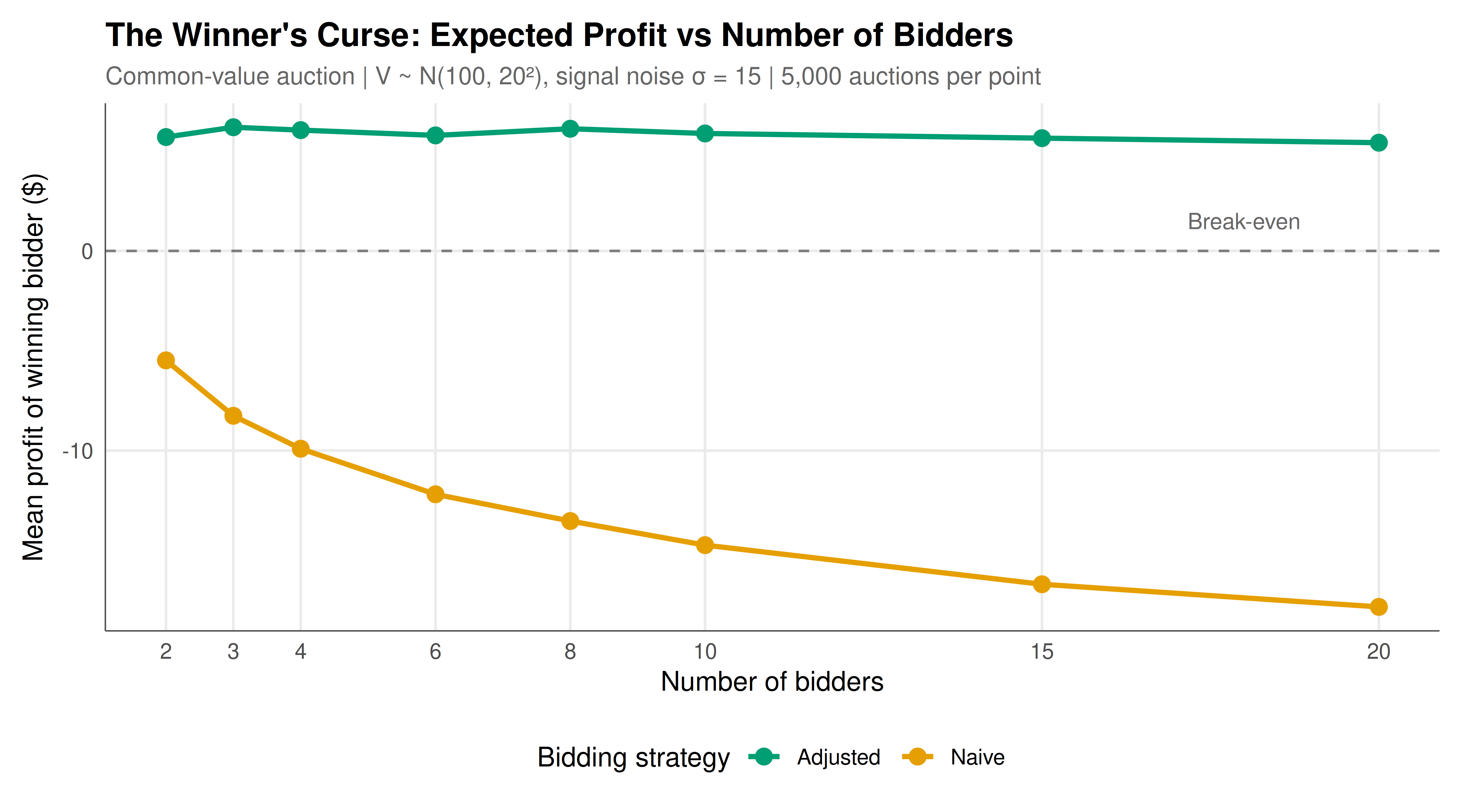
#| fig-cap: "The winner's curse intensifies with competition. Naive bidders (orange) earn increasingly negative profits as the number of bidders grows, while adjusted bidders (teal) maintain positive expected profits by shading their bids to account for the information content of winning."
#| fig-width: 9
#| fig-height: 5
#| dev: [png, pdf]
#| dpi: 300
ggplot(curse_by_n, aes(x = n_bidders, y = mean_profit, color = strategy)) +
  geom_line(linewidth = 1.1) +
  geom_point(size = 3) +
  geom_hline(yintercept = 0, linetype = "dashed", color = "grey50") +
  annotate("text", x = 18, y = 1.5, label = "Break-even", color = "grey40", size = 3.5) +
  scale_color_manual(values = c("Adjusted" = okabe_ito[3], "Naive" = okabe_ito[1])) +
  scale_x_continuous(breaks = bidder_counts) +
  labs(
    title = "The Winner's Curse: Expected Profit vs Number of Bidders",
    subtitle = sprintf("Common-value auction | V ~ N(%.0f, %.0f\u00b2), signal noise \u03c3 = %.0f | %s auctions per point",
                        mu_0, sigma_0, sigma_eps, format(5000, big.mark = ",")),
    x = "Number of bidders",
    y = "Mean profit of winning bidder ($)",
    color = "Bidding strategy"
  ) +
  theme_publication()
```
## Interactive figure
```{r}
#| label: fig-winners-curse-interactive
#| fig-cap: "Interactive exploration of profit distributions. Hover to compare mean profit and loss frequency for naive vs adjusted bidding strategies across different numbers of bidders."
curse_interactive <- curse_by_n |>
  mutate(
    text_label = sprintf(
      "Bidders: %d\nStrategy: %s\nMean Profit: $%.2f\nLoss Frequency: %.1f%%",
      n_bidders, strategy, mean_profit, pct_loss
    )
  )

p_int <- ggplot(curse_interactive,
                aes(x = n_bidders, y = mean_profit, color = strategy, text = text_label)) +
  geom_line(linewidth = 0.9) +
  geom_point(size = 2.5) +
  geom_hline(yintercept = 0, linetype = "dashed", color = "grey50") +
  scale_color_manual(values = c("Adjusted" = okabe_ito[3], "Naive" = okabe_ito[1])) +
  labs(
    title = "Winner's Curse by Competition Level",
    x = "Number of Bidders",
    y = "Mean Profit ($)",
    color = "Strategy"
  ) +
  theme_publication()

ggplotly(p_int, tooltip = "text") |>
  config(displaylogo = FALSE)
```
## Interpretation
The simulation results provide a stark and quantitative illustration of the winner's curse and the value of Bayesian reasoning in competitive bidding. The naive bidding strategy, which sets the bid equal to the posterior mean of the common value given one's own signal, produces systematically negative expected profits. This is not because the posterior mean is a biased estimator of the common value --- it is not --- but because the posterior mean fails to account for the selection effect inherent in winning a competitive auction. The winner of a first-price auction is, by definition, the bidder with the highest bid, which in symmetric equilibrium corresponds to the bidder with the highest signal. The highest signal among $n$ independent draws from the signal distribution is, on average, above the true value, because the maximum of $n$ random variables is a biased estimator of their common mean when $n > 1$. The larger $n$ is, the more extreme this upward bias becomes, which explains why the winner's curse intensifies with competition.
The numerical results make the magnitude of this effect concrete. With 6 bidders and our parameter values ($\mu_0 = 100$, $\sigma_0 = 20$, $\sigma_\varepsilon = 15$), naive bidders earn average profits substantially below zero, and more than half of winning bids result in losses (the winning bid exceeds the true common value). By the time we reach 20 bidders, the naive strategy is devastatingly unprofitable: the expected loss per auction is large, and the vast majority of wins result in overpayment. This pattern matches the empirical findings from oil lease auctions and laboratory experiments, where inexperienced bidders consistently lose money in common-value settings with moderate numbers of competitors.
The adjusted bidding strategy, which shades the bid downward by an amount proportional to the expected winner's curse, demonstrates the power of correct Bayesian reasoning. By bidding $E[V \mid X_i = x_i, X_i = X_{(n)}]$ rather than $E[V \mid X_i = x_i]$, the adjusted bidder incorporates the information content of winning into their valuation and avoids systematic overpayment. The simulation shows that adjusted bidders maintain positive expected profits across all competition levels, though the expected profit declines as the number of bidders increases (because competition drives bids closer to the true value). The adjustment is larger when there are more bidders, because the maximum order statistic is more extreme relative to the mean.
The Bayesian framework reveals the deep informational structure of the problem. In a common-value auction, the bidders' signals are not merely noise around a known value; they are pieces of information that, if pooled, would reveal the value more precisely. The auction mechanism aggregates this information, but it does so in a way that creates an adverse selection problem for the winner. The winner is the bidder who received the most favourable signal, which is also the signal most likely to be an overestimate. This is structurally identical to the lemons problem in used car markets (Akerlof 1970): the car you are offered is likely to be of lower quality than the average car, because better cars are less likely to be for sale. In auctions, the item you win is likely to be worth less than your estimate, because you would not have won if your estimate had not been unusually high.
The practical implications extend well beyond oil leases. The winner's curse affects any competitive bidding situation with common-value elements: takeover battles in corporate finance (where the target company's value is uncertain and common to all acquirers), procurement auctions (where the cost of a project is uncertain and affects all bidders similarly), and even online advertising auctions (where the click-through rate of an ad placement is common to advertisers in the same category). In each case, the winning bidder must ask: "Given that I am winning, what does that tell me about the value?" If the answer is "nothing good," then the bid should be shaded accordingly.
The pedagogical lesson is also important. The winner's curse is a natural setting for teaching Bayesian reasoning, because the conditional probability calculation is not merely an abstract exercise but has direct dollar consequences. Students who learn to compute the posterior mean given both their signal and the event of winning gain a visceral understanding of why conditioning matters and how failing to condition on relevant information (in this case, the information revealed by winning) leads to systematically biased decisions. This connects to broader themes in Bayesian inference, where conditioning on the observation process --- the "data you did not see" --- is essential for correct inference.
## Extensions and related tutorials
- **First-price and second-price auction theory** establish the revenue equivalence theorem for private-value auctions; see [Auction Theory Foundations](../../auction-theory-deep-dive/first-price-second-price/).
- **Bayesian Nash equilibrium** extends equilibrium analysis to games of incomplete information; see [Bayesian Games](../../foundations/bayesian-games/).
- **Mechanism design for revenue maximisation** derives optimal auction formats; see [Optimal Auction Design](../../mechanism-design/optimal-auctions/).
- **Spectrum auction design** applies these principles to real-world policy; see [Spectrum Auctions](../../case-studies/spectrum-auctions-policy/).
- **Prospect theory and behavioural bidding** models how real bidders deviate from Bayesian optimality; see [Endowment Effect and Exchange](../../behavioral-economics/endowment-effect-exchange/).
## References
::: {#refs}
:::