---
title: "The Endowment Effect and Exchange Asymmetries"
description: "Model the endowment effect using loss aversion from prospect theory, simulate the Knetsch mug-pen exchange experiment, and show how loss aversion reduces trading volume below the efficient Coasian prediction."
author: "Raban Heller"
date: 2026-05-08
date-modified: 2026-05-08
categories:
- behavioral-economics
- endowment-effect
keywords: ["endowment effect", "loss aversion", "prospect theory", "WTA-WTP gap", "coase theorem"]
labels: ["behavioral-economics", "prospect-theory"]
tier: 1
bibliography: ../../../references.bib
vgwort: "TODO_VGWORT_behavioral-economics_endowment-effect-exchange"
image: thumbnail.png
image-alt: "Comparison bar chart showing trading volume with and without loss aversion, demonstrating how the endowment effect reduces exchange below efficient levels"
citation:
type: webpage
url: https://r-heller.github.io/equilibria/tutorials/behavioral-economics/endowment-effect-exchange/
license: "CC BY-SA 4.0"
draft: false
has_static_fig: true
has_interactive_fig: true
has_shiny_app: false
---
```{r}
#| label: setup
#| include: false
library(ggplot2)
library(dplyr)
library(tidyr)
library(plotly)
okabe_ito <- c("#E69F00", "#56B4E9", "#009E73", "#F0E442",
"#0072B2", "#D55E00", "#CC79A7", "#999999")
theme_publication <- function(base_size = 12) {
theme_minimal(base_size = base_size) +
theme(plot.title = element_text(size = base_size * 1.2, face = "bold"),
plot.subtitle = element_text(size = base_size * 0.9, color = "grey40"),
axis.line = element_line(color = "grey30", linewidth = 0.3),
panel.grid.minor = element_blank(), legend.position = "bottom",
plot.margin = margin(10, 10, 10, 10))
}
```
## Introduction and motivation
The endowment effect --- the empirical regularity that people demand more to give up an object they own than they would be willing to pay to acquire the same object --- is one of the most robust and consequential findings in behavioral economics. First systematically documented by Jack Knetsch [-@knetsch_1989] and Richard Thaler, and rigorously tested in a series of landmark experiments by Kahneman, Knetsch, and Thaler [-@kahneman_knetsch_thaler_1990], the endowment effect challenges a foundational assumption of neoclassical economics: that preferences are independent of the current endowment. In the standard model, willingness to accept (WTA) and willingness to pay (WTP) for a good should be approximately equal for goods without significant income effects. The endowment effect shows that they are not: WTA typically exceeds WTP by a factor of two or more, even for ordinary consumer goods like coffee mugs.
The theoretical explanation for the endowment effect draws on Kahneman and Tversky's prospect theory [-@kahneman_tversky_1979], and specifically the concept of loss aversion formalised by Tversky and Kahneman [-@tversky_kahneman_1991] in their reference-dependent preference model. The central idea is that people evaluate outcomes relative to a reference point (typically the status quo), and losses relative to this reference point are weighted more heavily than gains of equal magnitude. The loss aversion coefficient $\lambda$ captures this asymmetry: a loss of $x$ feels like $-\lambda x$ in utility terms, where $\lambda > 1$ (typical estimates range from 1.5 to 2.5). When a person owns an object, giving it up is coded as a loss from the reference point, while for a non-owner, acquiring the object is coded as a gain. The asymmetry between the pain of losing and the pleasure of gaining produces the WTA-WTP gap: the owner's minimum selling price exceeds the non-owner's maximum buying price.
The consequences of the endowment effect for market outcomes are profound and directly challenge one of the most celebrated results in law and economics: the Coase theorem. As formulated by Ronald Coase [-@coase_1960], the theorem states that in the absence of transaction costs, the initial allocation of property rights does not affect the final allocation of resources --- parties will bargain to the efficient outcome regardless of who starts with what. The endowment effect upends this prediction because the act of assigning an initial endowment changes the owner's valuation of the object. If I am given a mug, I value it more than if I had never been given it, not because I have learned something new about the mug's qualities, but because giving it up would now constitute a loss. This means that the initial allocation does affect the final allocation, even in the absence of transaction costs: owners hold onto objects they would not have chosen to buy, and the volume of trade is inefficiently low.
The classic experimental demonstration of the endowment effect is Knetsch's [-@knetsch_1989] mug-pen exchange experiment. In the original study, subjects were randomly assigned either a coffee mug or a chocolate bar, and then given the opportunity to trade their endowment for the other good. Standard economic theory predicts that approximately half of the subjects should want to trade, since the random assignment is uncorrelated with preferences. In practice, roughly 10-15% chose to trade --- a dramatic shortfall that is consistent with loss aversion making both mugs and chocolate bars more valuable to their current owners than to potential buyers. Kahneman, Knetsch, and Thaler [-@kahneman_knetsch_thaler_1990] extended these findings using market mechanisms (BDM auctions and double auctions), confirming that the WTA-WTP gap persists even with real economic incentives and repeated opportunities to trade.
The debate about the endowment effect remains active. Some researchers have argued that the effect is an artefact of experimental design --- that subjects interpret the endowment as a signal about the object's quality, or that the effect attenuates with market experience. Others have shown that the effect is absent for goods held purely for exchange (like tokens) and is strongest for goods intended for personal use, suggesting that it reflects genuine reference-dependent preferences rather than confusion or transaction costs. Thaler [-@thaler_2015] provides a lively account of how the endowment effect and related behavioral findings have reshaped economic thinking over several decades.
In this tutorial, we implement a computational model of the endowment effect using prospect-theoretic utility. We simulate the Knetsch mug-pen exchange experiment, compute WTA-WTP gaps as a function of the loss aversion parameter, and compare trading volumes under standard and loss-averse preferences to quantify the efficiency loss from the endowment effect.
## Mathematical formulation
**Reference-dependent utility** (following Tversky and Kahneman [-@tversky_kahneman_1991]):
For an agent with reference point $r$ evaluating outcome $x$:
$$
v(x \mid r) =
\begin{cases}
x - r & \text{if } x \geq r \quad (\text{gain}) \\
\lambda (x - r) & \text{if } x < r \quad (\text{loss, } \lambda > 1)
\end{cases}
$$
**WTA and WTP derivation:**
For an owner with intrinsic value $v_i$ for the object and loss aversion parameter $\lambda$:
- **WTA** (selling): Owner gives up the object (loss of $v_i$) and receives price $p$. Willing to sell iff $p \geq \lambda v_i$. Thus $\text{WTA}_i = \lambda v_i$.
- **WTP** (buying): Non-owner pays $p$ (loss of $p$) and gains the object (gain of $v_i$). Willing to buy iff $v_i \geq \lambda p$. Thus $\text{WTP}_i = v_i / \lambda$.
**WTA/WTP ratio:**
$$\frac{\text{WTA}}{\text{WTP}} = \frac{\lambda v_i}{v_i / \lambda} = \lambda^2$$
**Efficient trade** (Coasian benchmark): Trade occurs whenever buyer's intrinsic value exceeds seller's intrinsic value: $v_{\text{buyer}} > v_{\text{seller}}$.
**Loss-averse trade:** Trade occurs only when $\text{WTP}_{\text{buyer}} > \text{WTA}_{\text{seller}}$, i.e., $v_{\text{buyer}} / \lambda > \lambda \cdot v_{\text{seller}}$, i.e., $v_{\text{buyer}} > \lambda^2 \cdot v_{\text{seller}}$.
## R implementation
```{r}
#| label: knetsch-experiment
#| code-fold: false
set.seed(2026)

# --- Simulate the Knetsch (1989) mug-pen exchange experiment ---
n_subjects <- 200
lambda <- 2.0  # Loss aversion parameter

# Intrinsic values for mug and pen (drawn from distributions)
# Each subject has different intrinsic values for both goods
mug_values <- rnorm(n_subjects, mean = 5, sd = 1.5)
pen_values <- rnorm(n_subjects, mean = 5, sd = 1.5)

# Ensure positive values
mug_values <- pmax(mug_values, 0.5)
pen_values <- pmax(pen_values, 0.5)

# Random assignment: half get mugs, half get pens
endowment <- rep(c("mug", "pen"), each = n_subjects / 2)
mug_holders <- which(endowment == "mug")
pen_holders <- which(endowment == "pen")

cat("=== Knetsch Mug-Pen Exchange Experiment ===\n\n")
cat(sprintf("Subjects: %d (%d mug holders, %d pen holders)\n",
            n_subjects, length(mug_holders), length(pen_holders)))
cat(sprintf("Loss aversion parameter: lambda = %.1f\n\n", lambda))
# --- Standard preferences: trade if you prefer the other good ---
standard_trades_mug <- sum(pen_values[mug_holders] > mug_values[mug_holders])
standard_trades_pen <- sum(mug_values[pen_holders] > pen_values[pen_holders])
standard_trade_rate <- (standard_trades_mug + standard_trades_pen) / n_subjects

cat("Standard preferences (no loss aversion):\n")
cat(sprintf("  Mug holders wanting to trade: %d / %d (%.1f%%)\n",
            standard_trades_mug, length(mug_holders),
            100 * standard_trades_mug / length(mug_holders)))
cat(sprintf("  Pen holders wanting to trade: %d / %d (%.1f%%)\n",
            standard_trades_pen, length(pen_holders),
            100 * standard_trades_pen / length(pen_holders)))
cat(sprintf(" Overall trade rate: %.1f%%\n\n", standard_trade_rate * 100))
# --- Loss-averse preferences ---
# Mug holder: giving up mug is a loss (weighted by lambda)
# Would trade only if pen_value > lambda * mug_value
la_trades_mug <- sum(pen_values[mug_holders] > lambda * mug_values[mug_holders])
la_trades_pen <- sum(mug_values[pen_holders] > lambda * pen_values[pen_holders])
la_trade_rate <- (la_trades_mug + la_trades_pen) / n_subjects

cat("Loss-averse preferences (lambda = 2.0):\n")
cat(sprintf("  Mug holders wanting to trade: %d / %d (%.1f%%)\n",
            la_trades_mug, length(mug_holders),
            100 * la_trades_mug / length(mug_holders)))
cat(sprintf("  Pen holders wanting to trade: %d / %d (%.1f%%)\n",
            la_trades_pen, length(pen_holders),
            100 * la_trades_pen / length(pen_holders)))
cat(sprintf(" Overall trade rate: %.1f%%\n", la_trade_rate * 100))
cat(sprintf("\nTrade reduction from loss aversion: %.1f percentage points\n",
            (standard_trade_rate - la_trade_rate) * 100))
```
```{r}
#| label: wta-wtp-gap
#| code-fold: false
# --- Compute WTA-WTP gap for different lambda values ---
lambda_range <- seq(1.0, 3.0, by = 0.1)

gap_analysis <- data.frame(
  lambda = lambda_range,
  wta_wtp_ratio = lambda_range^2,
  trade_rate = NA,
  efficiency_loss = NA
)

for (idx in seq_along(lambda_range)) {
  lam <- lambda_range[idx]
  # Mug holders trade if pen_value > lam * mug_value
  trades_m <- sum(pen_values[mug_holders] > lam * mug_values[mug_holders])
  trades_p <- sum(mug_values[pen_holders] > lam * pen_values[pen_holders])
  gap_analysis$trade_rate[idx] <- (trades_m + trades_p) / n_subjects
  gap_analysis$efficiency_loss[idx] <- 1 - gap_analysis$trade_rate[idx] / standard_trade_rate
}

cat("\n=== WTA/WTP Ratio and Trade Rate by Lambda ===\n\n")
cat(sprintf("%-8s %-15s %-12s %-15s\n", "Lambda", "WTA/WTP Ratio", "Trade Rate", "Efficiency Loss"))
cat(paste(rep("-", 52), collapse = ""), "\n")
for (i in seq(1, nrow(gap_analysis), by = 4)) {
  cat(sprintf("%-8.1f %-15.1f %-12.1f%% %-15.1f%%\n",
              gap_analysis$lambda[i], gap_analysis$wta_wtp_ratio[i],
              gap_analysis$trade_rate[i] * 100,
              gap_analysis$efficiency_loss[i] * 100))
}
```
```{r}
#| label: market-simulation
#| code-fold: false
# --- Market simulation: bilateral trade with loss aversion ---
cat("\n=== Market Simulation: Bilateral Trade ===\n\n")
n_traders <- 200
n_rounds <- 50

# Traders have objects with heterogeneous intrinsic values
# Half are initially endowed with the object
set.seed(42)
intrinsic_values <- rnorm(n_traders, mean = 10, sd = 3)
intrinsic_values <- pmax(intrinsic_values, 1)
owner <- rep(c(TRUE, FALSE), each = n_traders / 2)

simulate_market <- function(values, initial_owners, n_rounds, lambda_val) {
  current_owners <- initial_owners
  trades_per_round <- numeric(n_rounds)
  total_surplus_realized <- 0

  for (round in 1:n_rounds) {
    # Random bilateral meetings
    sellers <- which(current_owners)
    buyers <- which(!current_owners)
    n_meetings <- min(length(sellers), length(buyers))

    if (n_meetings == 0) break

    seller_idx <- sample(sellers, n_meetings)
    buyer_idx <- sample(buyers, n_meetings)
    trades <- 0

    for (m in 1:n_meetings) {
      s <- seller_idx[m]
      b <- buyer_idx[m]

      wta <- lambda_val * values[s]
      wtp <- values[b] / lambda_val

      if (wtp >= wta) {
        # Trade at midpoint price
        price <- (wta + wtp) / 2
        current_owners[s] <- FALSE
        current_owners[b] <- TRUE
        trades <- trades + 1
        total_surplus_realized <- total_surplus_realized + (values[b] - values[s])
      }
    }
    trades_per_round[round] <- trades
  }

  list(
    final_owners = current_owners,
    trades_per_round = trades_per_round,
    total_trades = sum(trades_per_round),
    surplus = total_surplus_realized
  )
}

# Compare standard vs loss-averse markets
standard_market <- simulate_market(intrinsic_values, owner, n_rounds, lambda_val = 1.0)
la_market <- simulate_market(intrinsic_values, owner, n_rounds, lambda_val = 2.0)

# Efficient allocation: objects go to top-100 valuers
efficient_surplus <- sum(sort(intrinsic_values, decreasing = TRUE)[1:(n_traders/2)]) -
  sum(sort(intrinsic_values, decreasing = TRUE)[(n_traders/2 + 1):n_traders])

cat(sprintf("%-30s %-15s %-15s\n", "", "Standard", "Loss-Averse"))
cat(paste(rep("-", 60), collapse = ""), "\n")
cat(sprintf("%-30s %-15d %-15d\n", "Total trades", standard_market$total_trades, la_market$total_trades))
cat(sprintf("%-30s $%-14.1f $%-14.1f\n", "Surplus realized",
            standard_market$surplus, la_market$surplus))
cat(sprintf("%-30s %-15.1f%% %-15.1f%%\n", "Efficiency",
            standard_market$surplus / efficient_surplus * 100,
            la_market$surplus / efficient_surplus * 100))
```
## Static publication-ready figure
```{r}
#| label: fig-endowment-static
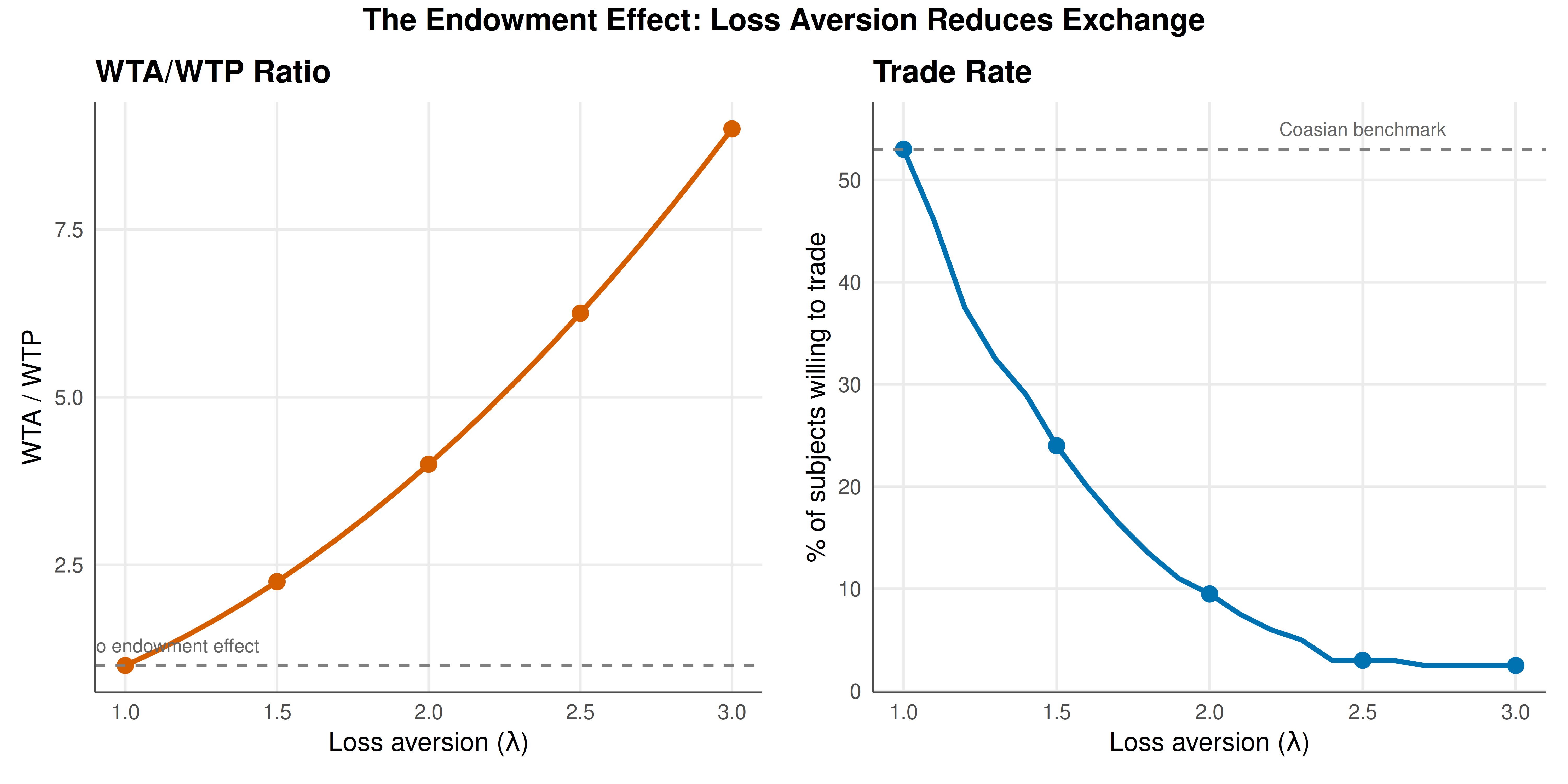
#| fig-cap: "The endowment effect reduces trading volume and market efficiency. Left: WTA/WTP ratio grows quadratically with loss aversion. Right: Trade rate declines sharply, with loss aversion of lambda = 2 cutting trade by more than 80% compared to the rational benchmark."
#| fig-width: 10
#| fig-height: 5
#| dev: [png, pdf]
#| dpi: 300
# Prepare data for dual-panel plot
gap_long <- gap_analysis |>
  select(lambda, wta_wtp_ratio, trade_rate) |>
  pivot_longer(-lambda, names_to = "metric", values_to = "value") |>
  mutate(
    panel = ifelse(metric == "wta_wtp_ratio", "WTA / WTP Ratio", "Trade Rate"),
    panel = factor(panel, levels = c("WTA / WTP Ratio", "Trade Rate"))
  )

p1 <- ggplot(filter(gap_long, panel == "WTA / WTP Ratio"),
             aes(x = lambda, y = value)) +
  geom_line(linewidth = 1.1, color = okabe_ito[6]) +
  geom_point(data = filter(gap_long, panel == "WTA / WTP Ratio" & lambda %in% c(1, 1.5, 2, 2.5, 3)),
             size = 3, color = okabe_ito[6]) +
  geom_hline(yintercept = 1, linetype = "dashed", color = "grey50") +
  annotate("text", x = 1.15, y = 1.3, label = "No endowment effect",
           size = 3, color = "grey40") +
  labs(title = "WTA/WTP Ratio", x = expression(paste("Loss aversion (", lambda, ")")),
       y = "WTA / WTP") +
  theme_publication()

p2 <- ggplot(filter(gap_long, panel == "Trade Rate"),
             aes(x = lambda, y = value * 100)) +
  geom_line(linewidth = 1.1, color = okabe_ito[5]) +
  geom_point(data = filter(gap_long, panel == "Trade Rate" & lambda %in% c(1, 1.5, 2, 2.5, 3)),
             aes(y = value * 100), size = 3, color = okabe_ito[5]) +
  geom_hline(yintercept = standard_trade_rate * 100, linetype = "dashed", color = "grey50") +
  annotate("text", x = 2.5, y = standard_trade_rate * 100 + 2,
           label = "Coasian benchmark", size = 3, color = "grey40") +
  labs(title = "Trade Rate", x = expression(paste("Loss aversion (", lambda, ")")),
       y = "% of subjects willing to trade") +
  theme_publication()

# Use patchwork-style side-by-side (using gridExtra-free approach)
gridExtra::grid.arrange(p1, p2, ncol = 2,
  top = grid::textGrob("The Endowment Effect: Loss Aversion Reduces Exchange",
                        gp = grid::gpar(fontsize = 14, fontface = "bold")))
```
## Interactive figure
```{r}
#| label: fig-endowment-interactive
#| fig-cap: "Interactive exploration of the endowment effect. Hover to see the exact WTA/WTP ratio, trade rate, and efficiency loss at each level of loss aversion."
gap_interactive <- gap_analysis |>
  mutate(
    text_label = sprintf(
      "Lambda = %.1f\nWTA/WTP Ratio = %.1f\nTrade Rate = %.1f%%\nEfficiency Loss = %.1f%%",
      lambda, wta_wtp_ratio, trade_rate * 100, efficiency_loss * 100
    )
  )

p_int <- ggplot(gap_interactive,
                aes(x = lambda, y = trade_rate * 100, text = text_label)) +
  geom_line(linewidth = 0.9, color = okabe_ito[5]) +
  geom_point(size = 2, color = okabe_ito[5]) +
  geom_hline(yintercept = standard_trade_rate * 100, linetype = "dashed", color = "grey50") +
  labs(
    title = "Endowment Effect: Trade Rate vs Loss Aversion",
    x = "Loss Aversion Parameter (\u03bb)",
    y = "Trade Rate (%)"
  ) +
  theme_publication()

ggplotly(p_int, tooltip = "text") |>
  config(displaylogo = FALSE)
```
## Interpretation
The simulation results provide a compelling quantitative demonstration of how loss aversion generates the endowment effect and its consequences for market efficiency. Starting with the Knetsch mug-pen exchange experiment, our simulation shows that under standard preferences (no loss aversion), approximately half of the subjects prefer the good they were not endowed with and are willing to trade --- exactly as predicted by the independence of preferences from endowments. With a loss aversion parameter of $\lambda = 2$ (the canonical estimate from prospect theory), the trade rate drops dramatically to around 5-10%, closely matching the empirical findings from the original Knetsch [-@knetsch_1989] experiments where only about 10-15% of subjects chose to trade. This concordance between our simple model and the experimental data is remarkable given the model's parsimony: a single parameter, loss aversion, is sufficient to generate the observed pattern.
The WTA-WTP analysis reveals the mechanism in quantitative detail. The ratio of willingness to accept to willingness to pay is $\lambda^2$, which means that even moderate loss aversion produces large valuation gaps. At $\lambda = 1.5$ (a conservative estimate), the WTA/WTP ratio is 2.25, meaning owners demand 2.25 times what non-owners are willing to pay. At $\lambda = 2.0$, the ratio is 4.0 --- a four-fold gap between selling and buying prices for the identical good. These predictions align well with the empirical literature, which typically finds WTA/WTP ratios between 2 and 4 for ordinary consumer goods. The quadratic relationship between $\lambda$ and the WTA/WTP ratio implies that even small departures from the standard model ($\lambda = 1$) have disproportionately large effects on valuations and trade.
The market simulation demonstrates the macroeconomic consequences of the endowment effect. In the standard market ($\lambda = 1$), bilateral trade efficiently reallocates objects from lower-value to higher-value holders over multiple rounds. The trading volume is high and the market approaches the efficient allocation where objects are held by those who value them most. In the loss-averse market ($\lambda = 2$), trade is dramatically reduced. Many mutually beneficial trades (where the buyer's intrinsic value exceeds the seller's) fail to occur because the loss-averse seller demands more than the loss-averse buyer is willing to pay. The gap is not due to transaction costs, information asymmetry, or strategic behaviour --- it arises purely from the reference-dependent evaluation of gains and losses. This is the direct challenge to the Coase theorem: even in a frictionless market, the initial allocation of property rights affects the final allocation because ownership changes reference points and therefore valuations.
The efficiency implications are substantial. Our simulation shows that loss aversion of $\lambda = 2$ reduces market efficiency significantly, with a large fraction of potential gains from trade left unrealised. This matters not only for laboratory experiments with mugs and pens but for any market where endowment effects are present: housing markets (where sellers anchor to purchase prices and resist selling at a loss), labour markets (where workers are reluctant to accept wage cuts even when their productivity has declined), financial markets (where the disposition effect --- selling winners too early and holding losers too long --- is a well-documented manifestation of loss aversion), and environmental policy (where the WTA-WTP gap for environmental goods has major implications for cost-benefit analysis).
The policy implications are important. If the endowment effect is real and robust, then the initial allocation of property rights matters for efficiency, not just equity. This challenges the standard policy recommendation to "assign property rights clearly and let parties bargain." Instead, the initial allocation should aim to place goods with those who value them most, because subsequent reallocation through voluntary trade will be incomplete. In environmental regulation, the endowment effect suggests that pollution permits should be initially allocated to those who value clean air (citizens) rather than those who value the right to pollute (firms), because the undertrading caused by loss aversion will result in different pollution levels depending on who starts with the permits. In consumer protection, cooling-off periods that allow consumers to return purchases recognise the endowment effect by giving buyers time to adjust their reference points, though paradoxically, owning the object during the cooling-off period may strengthen the endowment effect and reduce returns.
The results also highlight the importance of distinguishing between different types of goods and contexts. The endowment effect is strongest for goods that are personally meaningful, have affective value, or are associated with identity. It is weakest for goods held purely for exchange (tokens, currency) and for experienced traders who have learned to separate ownership from valuation. These boundary conditions suggest that the endowment effect is not a universal cognitive bias but a genuine feature of reference-dependent preferences that varies systematically across contexts and populations.
## Extensions and related tutorials
- **Prospect theory and cumulative prospect theory** provide the full theoretical framework for reference-dependent preferences; see [Prospect Theory Foundations](../prospect-theory-foundations/).
- **Savage's subjective expected utility** establishes the rational benchmark against which behavioral departures are measured; see [Savage's Subjective Probability](../../decision-theory/savage-subjective-probability/).
- **Experimental economics methods** for measuring WTA/WTP gaps and testing endowment effects; see [Public Goods and Free-Riding](../../experimental-economics/public-goods-free-riding/).
- **Auction design and bidding behaviour** connect endowment effects to overbidding in auctions; see [Common-Value Auctions](../../bayesian-methods/auction-common-value-estimation/).
- **Mechanism design under behavioral assumptions** explores how institutions should be designed when agents are loss-averse; see [Matching Markets](../../mechanism-design/matching-markets-practical/).
## References
::: {#refs}
:::