---
title: "Bayesian persuasion and information design"
description: "Implement the Kamenica-Gentzkow (2011) Bayesian persuasion model in R, computing optimal signal structures via concavification for the binary-state prosecutor-judge example."
author: "Raban Heller"
date: 2026-05-08
date-modified: 2026-05-08
categories:
- bayesian-methods
- information-design
- bayesian-persuasion
- signalling
keywords: ["Bayesian persuasion", "information design", "concavification", "Kamenica Gentzkow", "optimal signalling"]
labels: ["information-economics", "mechanism-design"]
tier: 1
bibliography: ../../../references.bib
vgwort: "TODO_VGWORT_bayesian-methods_information-design-persuasion"
image: thumbnail.png
image-alt: "Concavification plot showing the sender's value function and its concave closure for Bayesian persuasion"
citation:
type: webpage
url: https://r-heller.github.io/equilibria/tutorials/bayesian-methods/information-design-persuasion/
license: "CC BY-SA 4.0"
draft: false
has_static_fig: true
has_interactive_fig: true
has_shiny_app: false
---
```{r}
#| label: setup
#| include: false
library(ggplot2)
library(dplyr)
library(tidyr)
library(plotly)
okabe_ito <- c("#E69F00", "#56B4E9", "#009E73", "#F0E442",
"#0072B2", "#D55E00", "#CC79A7", "#999999")
theme_publication <- function(base_size = 12) {
theme_minimal(base_size = base_size) +
theme(plot.title = element_text(size = base_size * 1.2, face = "bold"),
plot.subtitle = element_text(size = base_size * 0.9, color = "grey40"),
axis.line = element_line(color = "grey30", linewidth = 0.3),
panel.grid.minor = element_blank(), legend.position = "bottom",
plot.margin = margin(10, 10, 10, 10))
}
```
## Introduction & motivation
Information is power — but how exactly does the control of information translate into strategic advantage? In many economic, legal, and political settings, one party (the "sender") has the ability to design what information another party (the "receiver") observes before making a decision. A prosecutor chooses which evidence to present to a judge. A pharmaceutical company designs clinical trials whose results regulators will see. A central bank crafts its communication strategy to influence market expectations. A lobbyist commissions studies to present to a legislator. In all these cases, the sender cannot fabricate information — the evidence must be truthful — but the sender can choose what experiments to run, what questions to ask, or what data to reveal. The fundamental insight of Bayesian persuasion, formalised by Kamenica and Gentzkow (2011), is that this ability to design the information structure can be enormously valuable, even when the sender cannot lie and the receiver is fully rational.
The Bayesian persuasion framework models a game between a sender and a receiver. Nature first draws a state of the world $\omega$ from a known prior distribution. The sender commits to a signal structure (an experiment, an information policy) before observing the state; this signal structure specifies, for each possible state, a probability distribution over signals that will be sent to the receiver. After the state is realised, the signal is drawn according to the chosen structure and revealed to the receiver. The receiver then updates her beliefs using Bayes' rule and takes an action that maximises her expected utility given her posterior belief. The sender's payoff depends on the receiver's action (and possibly the state). The key constraint is that the signal must be Bayes-plausible: the expected posterior belief must equal the prior. The sender cannot systematically mislead the receiver, but she can strategically choose how much and what kind of information to reveal.
The central analytical tool for solving Bayesian persuasion problems is concavification. Kamenica and Gentzkow showed that the sender's optimal expected payoff from information design equals the value of the concave closure (or concavification) of the sender's value function evaluated at the prior. The value function $V(\mu)$ gives the sender's payoff when the receiver holds posterior belief $\mu$ and acts optimally. Because the receiver's optimal action changes discontinuously as beliefs cross certain thresholds, $V(\mu)$ is typically non-concave. The concave closure $\hat{V}(\mu)$ is the smallest concave function that lies weakly above $V(\mu)$ everywhere. If $\hat{V}(\mu_0) > V(\mu_0)$ at the prior $\mu_0$, the sender can strictly benefit from information design — she should design a signal that splits the prior into posterior beliefs where $V$ is higher, exploiting the non-concavity.
In this tutorial, we implement the complete Bayesian persuasion analysis for the canonical binary-state example: a prosecutor (sender) who wants a judge (receiver) to convict a defendant. The defendant is either guilty or innocent, and the judge convicts only if her posterior belief of guilt exceeds a threshold. Under the prior alone, the judge would acquit. The prosecutor cannot fabricate evidence but can choose how informative her investigation is — she designs a signal structure. We compute the sender's value function, perform the concavification, find the optimal signal, and verify that the resulting posteriors are Bayes-plausible. We then compare the sender's payoffs under no information, full information, and optimal information design, showing that the optimal signal achieves a strictly higher payoff than either extreme. The tutorial provides working R code for all computations and produces both a static publication-quality concavification diagram and an interactive figure.
The Bayesian persuasion framework has generated an enormous literature in economics since 2011, with extensions to multiple receivers, multiple senders, dynamic settings, and costly information acquisition. It has become a cornerstone of the field of information design, which studies how the provision of information affects strategic behaviour and market outcomes. Understanding the basic concavification approach is essential for engaging with this literature.
## Mathematical formulation
**Setup.** There are two states of the world $\omega \in \{G, I\}$ (Guilty, Innocent) with prior $\mu_0 = \Pr(\omega = G)$. The receiver (judge) chooses an action $a \in \{C, A\}$ (Convict, Acquit). The receiver's utility is:
$$
u_R(a, \omega) = \begin{cases} 1 & \text{if } a = C, \omega = G \\ -q & \text{if } a = C, \omega = I \\ 0 & \text{if } a = A \end{cases}
$$
where $q > 0$ is the cost of convicting an innocent person relative to the benefit of convicting a guilty one. The receiver convicts if and only if her posterior belief $\mu = \Pr(G \mid \text{signal})$ satisfies:
$$
\mu \cdot 1 + (1-\mu) \cdot (-q) \geq 0 \quad \Longleftrightarrow \quad \mu \geq \frac{q}{1+q} \equiv \bar{\mu}
$$
The sender (prosecutor) always prefers conviction: $u_S(C) = 1$, $u_S(A) = 0$.
**Value function.** The sender's value function maps the receiver's posterior to the sender's expected payoff:
$$
V(\mu) = \begin{cases} 1 & \text{if } \mu \geq \bar{\mu} \\ 0 & \text{if } \mu < \bar{\mu} \end{cases}
$$
**Signal structure.** A signal $\pi$ consists of a set of signal realisations $S$ and conditional distributions $\pi(\cdot \mid \omega)$. For binary states, any signal can be summarised by the posteriors it induces. A signal inducing posteriors $\mu_1$ and $\mu_2$ with probabilities $\lambda$ and $1-\lambda$ must satisfy Bayes plausibility:
$$
\lambda \mu_1 + (1 - \lambda) \mu_2 = \mu_0
$$
**Concavification.** The sender's optimal value is $\hat{V}(\mu_0)$, where $\hat{V}$ is the concave closure of $V$:
$$
\hat{V}(\mu_0) = \sup \left\{ \sum_s \lambda_s V(\mu_s) : \sum_s \lambda_s \mu_s = \mu_0, \; \lambda_s \geq 0, \; \sum_s \lambda_s = 1 \right\}
$$
For the binary case, concavification reduces to finding the upper concave envelope of $V(\mu)$ on $[0, 1]$.
**Optimal signal.** The optimal signal splits the prior $\mu_0$ into $\mu_L = 0$ (full exoneration) and $\mu_H = \bar{\mu}$ (just enough to convict), with:
$$
\lambda_H = \frac{\mu_0}{\bar{\mu}}, \quad \lambda_L = 1 - \frac{\mu_0}{\bar{\mu}}
$$
This yields sender payoff $\hat{V}(\mu_0) = \mu_0 / \bar{\mu} = \mu_0 (1+q) / q$.
## R implementation
```{r}
#| label: persuasion-implementation
set.seed(42)

# Parameters
mu0 <- 0.3      # Prior probability of guilty
q <- 1.5         # Cost of wrongful conviction
mu_bar <- q / (1 + q)  # Conviction threshold

cat(sprintf("Prior belief (mu_0): %.2f\n", mu0))
cat(sprintf("Conviction cost (q): %.2f\n", q))
cat(sprintf("Conviction threshold (mu_bar): %.4f\n", mu_bar))
cat(sprintf("Prior < threshold? %s => Judge acquits under prior alone\n\n",
            ifelse(mu0 < mu_bar, "YES", "NO")))
# Sender's value function
V <- function(mu) ifelse(mu >= mu_bar, 1, 0)

# Concave closure for binary case
V_hat <- function(mu) {
  ifelse(mu >= mu_bar, 1, mu / mu_bar)
}

# Optimal signal structure
lambda_H <- mu0 / mu_bar  # Prob of "convict" signal
lambda_L <- 1 - lambda_H  # Prob of "acquit" signal
mu_H <- mu_bar             # Posterior after "convict" signal
mu_L <- 0                  # Posterior after "acquit" signal

cat("=== Optimal Signal Structure ===\n")
cat(sprintf("Signal 'convict': posterior = %.4f, probability = %.4f\n",
            mu_H, lambda_H))
cat(sprintf("Signal 'acquit':  posterior = %.4f, probability = %.4f\n",
            mu_L, lambda_L))
# Verify Bayes plausibility
bp_check <- lambda_H * mu_H + lambda_L * mu_L
cat(sprintf("\nBayes plausibility check: %.4f * %.4f + %.4f * %.4f = %.4f (should = %.4f)\n",
            lambda_H, mu_H, lambda_L, mu_L, bp_check, mu0))
# Signal conditional probabilities
# pi(convict | G) and pi(convict | I)
# From Bayes rule: mu_H = pi(c|G) * mu0 / (pi(c|G)*mu0 + pi(c|I)*(1-mu0))
# And: lambda_H = pi(c|G)*mu0 + pi(c|I)*(1-mu0)
# Since mu_L = 0, we need pi(acquit|G) = 0, so pi(convict|G) = 1
pi_c_G <- 1
pi_c_I <- lambda_H * (1 - mu0) / (1 - mu0)  # simplification
# More carefully: lambda_H = pi_c_G * mu0 + pi_c_I * (1-mu0)
# pi_c_G = 1, so: pi_c_I = (lambda_H - mu0) / (1 - mu0)
pi_c_I <- (lambda_H - mu0) / (1 - mu0)

cat(sprintf("\nSignal conditional probabilities:\n"))
cat(sprintf(" pi(convict | Guilty) = %.4f\n", pi_c_G))
cat(sprintf(" pi(convict | Innocent) = %.4f\n", pi_c_I))
cat(sprintf(" pi(acquit | Guilty) = %.4f\n", 1 - pi_c_G))
cat(sprintf(" pi(acquit | Innocent) = %.4f\n", 1 - pi_c_I))
# Compare payoffs under different information regimes
payoff_no_info <- V(mu0)
payoff_full_info <- mu0 * V(1) + (1 - mu0) * V(0)
payoff_optimal <- V_hat(mu0)

cat(sprintf("\n=== Sender's Expected Payoff ===\n"))
cat(sprintf("No information (prior only): %.4f\n", payoff_no_info))
cat(sprintf("Full information: %.4f\n", payoff_full_info))
cat(sprintf("Optimal signal (persuasion): %.4f\n", payoff_optimal))
cat(sprintf("Gain from persuasion vs none: +%.4f\n", payoff_optimal - payoff_no_info))
cat(sprintf("Gain from persuasion vs full: +%.4f\n", payoff_optimal - payoff_full_info))
```
```{r}
#| label: comparative-statics
# How optimal payoff varies with prior and threshold
prior_grid <- seq(0, 1, by = 0.01)
q_values <- c(0.5, 1.0, 1.5, 2.0, 3.0)

cs_data <- expand.grid(mu0 = prior_grid, q = q_values) |>
  mutate(
    mu_bar = q / (1 + q),
    V_no_info = ifelse(mu0 >= mu_bar, 1, 0),
    V_full = mu0,
    V_optimal = ifelse(mu0 >= mu_bar, 1, mu0 / mu_bar),
    persuasion_value = V_optimal - pmax(V_no_info, V_full),
    q_label = paste0("q = ", q)
  )

cat("Persuasion value at prior = 0.3 for different q:\n")
cs_data |>
  filter(abs(mu0 - 0.3) < 0.005) |>
  select(q, mu_bar, V_no_info, V_full, V_optimal, persuasion_value) |>
  print()
```
## Static publication-ready figure
```{r}
#| label: fig-concavification
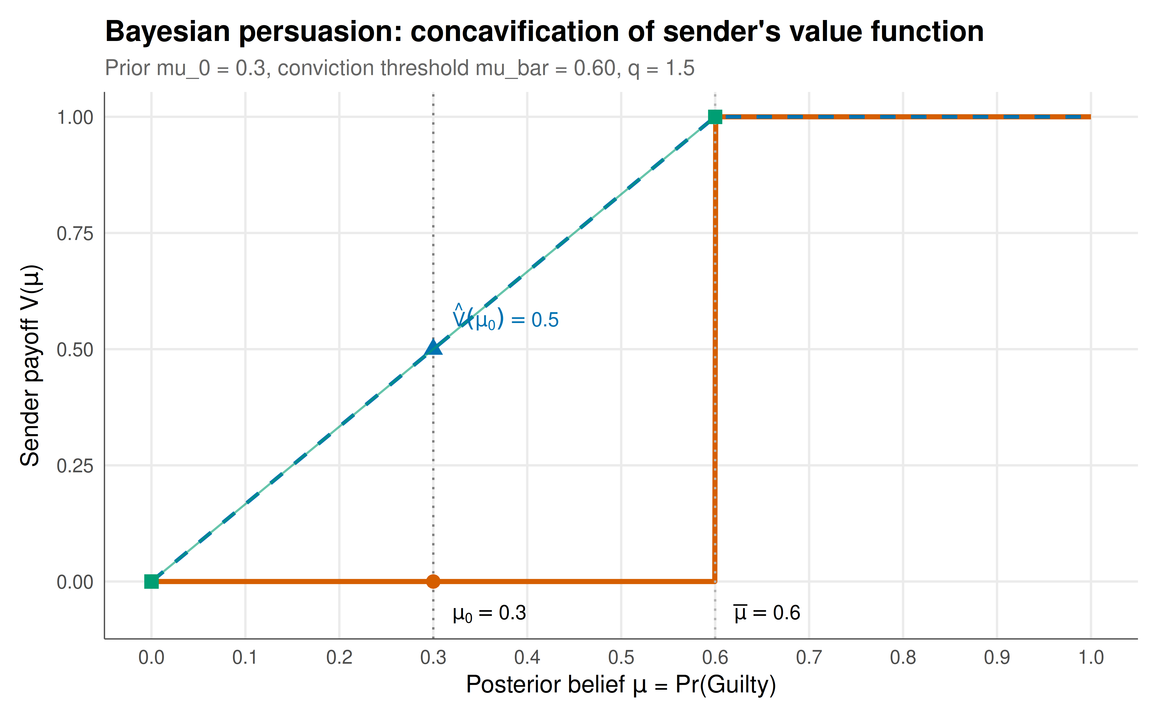
#| fig-cap: "Figure 1. Concavification for Bayesian persuasion. The step function V(mu) is the sender's payoff as a function of the receiver's posterior belief. The dashed line is the concave closure V-hat(mu). At the prior mu_0 = 0.3, the optimal signal splits the prior into posteriors 0 and mu_bar = 0.6, achieving sender payoff V-hat(mu_0) = 0.5 instead of V(mu_0) = 0. Okabe-Ito palette."
#| dev: [png, pdf]
#| fig-width: 8
#| fig-height: 5
#| dpi: 300
# Build plot data
mu_seq <- seq(0, 1, length.out = 1000)
plot_data <- data.frame(
  mu = mu_seq,
  V = V(mu_seq),
  V_hat = V_hat(mu_seq)
)

# Key points
key_points <- data.frame(
  mu = c(mu0, mu0, mu_L, mu_H),
  y = c(V(mu0), V_hat(mu0), V(mu_L), V(mu_H)),
  label = c("V(mu_0) = 0", sprintf("V_hat(mu_0) = %.2f", V_hat(mu0)),
            "mu_L = 0", sprintf("mu_H = %.2f", mu_bar)),
  type = c("original", "concavified", "posterior", "posterior")
)

p_concav <- ggplot() +
  # Value function (step)
  geom_line(data = plot_data, aes(x = mu, y = V),
            color = okabe_ito[6], linewidth = 1.2) +
  # Concave closure (dashed)
  geom_line(data = plot_data, aes(x = mu, y = V_hat),
            color = okabe_ito[5], linewidth = 0.9, linetype = "dashed") +
  # Prior vertical line
  geom_vline(xintercept = mu0, linetype = "dotted", color = "grey50") +
  # Threshold vertical line
  geom_vline(xintercept = mu_bar, linetype = "dotted", color = "grey70") +
  # Points

  geom_point(aes(x = mu0, y = V(mu0)), color = okabe_ito[6],
             size = 3, shape = 16) +
  geom_point(aes(x = mu0, y = V_hat(mu0)), color = okabe_ito[5],
             size = 3, shape = 17) +
  geom_point(aes(x = mu_L, y = V(mu_L)), color = okabe_ito[3],
             size = 3, shape = 15) +
  geom_point(aes(x = mu_H, y = V(mu_H)), color = okabe_ito[3],
             size = 3, shape = 15) +
  # Splitting line
  geom_segment(aes(x = mu_L, y = V(mu_L), xend = mu_H, yend = V(mu_H)),
               color = okabe_ito[3], linewidth = 0.5, linetype = "solid",
               alpha = 0.6) +
  # Annotations
  annotate("text", x = mu0 + 0.02, y = V_hat(mu0) + 0.07,
           label = sprintf("hat(V)(mu[0]) == %.2f", V_hat(mu0)),
           parse = TRUE, size = 3.5, hjust = 0, color = okabe_ito[5]) +
  annotate("text", x = mu0 + 0.02, y = -0.07,
           label = sprintf("mu[0] == %.1f", mu0),
           parse = TRUE, size = 3.5, hjust = 0) +
  annotate("text", x = mu_bar + 0.02, y = -0.07,
           label = sprintf("bar(mu) == %.2f", mu_bar),
           parse = TRUE, size = 3.5, hjust = 0) +
  scale_x_continuous(breaks = seq(0, 1, by = 0.1)) +
  labs(
    title = "Bayesian persuasion: concavification of sender's value function",
    subtitle = sprintf("Prior mu_0 = %.1f, conviction threshold mu_bar = %.2f, q = %.1f",
                       mu0, mu_bar, q),
    x = expression(paste("Posterior belief ", mu, " = Pr(Guilty)")),
    y = expression(paste("Sender payoff V(", mu, ")"))
  ) +
  theme_publication()

p_concav
```
## Interactive figure
```{r}
#| label: fig-persuasion-comparative-interactive
cs_plot <- cs_data |>
  filter(q %in% c(0.5, 1.5, 3.0)) |>
  select(mu0, q_label, V_no_info, V_full, V_optimal) |>
  pivot_longer(c(V_no_info, V_full, V_optimal),
               names_to = "regime", values_to = "payoff") |>
  mutate(
    regime = case_when(
      regime == "V_no_info" ~ "No information",
      regime == "V_full" ~ "Full information",
      regime == "V_optimal" ~ "Optimal persuasion"
    ),
    regime = factor(regime, levels = c("No information", "Full information",
                                        "Optimal persuasion")),
    text = sprintf("Prior: %.2f\nRegime: %s\nPayoff: %.3f\n%s",
                   mu0, regime, payoff, q_label)
  )

p_cs <- ggplot(cs_plot,
       aes(x = mu0, y = payoff, color = regime, text = text)) +
  geom_line(linewidth = 0.7) +
  facet_wrap(~q_label, nrow = 1) +
  scale_color_manual(values = c("No information" = okabe_ito[8],
                                 "Full information" = okabe_ito[1],
                                 "Optimal persuasion" = okabe_ito[5])) +
  labs(
    title = "Sender payoff across information regimes",
    x = expression(paste("Prior ", mu[0])),
    y = "Sender's expected payoff",
    color = "Information regime"
  ) +
  theme_publication() +
  theme(strip.text = element_text(face = "bold"))

ggplotly(p_cs, tooltip = "text") |>
  config(displaylogo = FALSE,
         modeBarButtonsToRemove = c("select2d", "lasso2d"))
```
## Interpretation
The concavification analysis reveals the core logic of Bayesian persuasion with striking clarity. When the prior probability of guilt is $\mu_0 = 0.3$ and the conviction threshold is $\bar{\mu} = 0.6$, the judge acquits under the prior — no information means the sender (prosecutor) gets a payoff of zero. Full revelation does better: with probability $\mu_0 = 0.3$ the state is Guilty, the judge sees this and convicts, giving the sender a payoff of 0.3. But the optimal signal does better still: it achieves a payoff of $\mu_0 / \bar{\mu} = 0.5$. The sender convicts 50% of the time, even though only 30% of defendants are actually guilty. This seemingly paradoxical result is not achieved through deception — the signal is honest and the judge is fully rational — but through strategic information design.
The mechanism works as follows. The optimal signal generates two outcomes: a "convict" signal that leaves the judge with posterior exactly $\bar{\mu} = 0.6$ (just enough to convict), and an "acquit" signal that leaves the judge with posterior $0$ (certain innocence). The key insight is that the "convict" signal is sent whenever the defendant is guilty ($\pi(\text{convict} \mid G) = 1$) and with some probability when the defendant is innocent ($\pi(\text{convict} \mid I) > 0$). This pooling of some innocent defendants with all guilty defendants is what allows the prosecutor to achieve a conviction rate higher than the base rate of guilt. The judge knows this is happening — she understands the signal structure — but she cannot improve her decision given her posterior belief. When she receives the "convict" signal, her belief of guilt is exactly $\bar{\mu}$, which makes her just indifferent between convicting and acquitting. The sender exploits this indifference.
The concavification diagram makes the geometry intuitive. The sender's value function $V(\mu)$ is a step function that jumps from 0 to 1 at $\bar{\mu}$. This function is not concave — the jump creates a "concavity gap." The concave closure $\hat{V}(\mu)$ fills in this gap by drawing a straight line from $(0, 0)$ to $(\bar{\mu}, 1)$. Any prior $\mu_0$ that falls in this gap (i.e., $\mu_0 < \bar{\mu}$) can benefit from persuasion: the sender achieves $\hat{V}(\mu_0) > V(\mu_0)$. The size of the gap — and hence the value of persuasion — depends on the conviction threshold $\bar{\mu}$, which in turn depends on the judge's cost parameter $q$. When $q$ is small (the judge does not care much about wrongful convictions), $\bar{\mu}$ is small and there is little room for persuasion. When $q$ is large (the judge is very cautious), $\bar{\mu}$ is large and the scope for persuasion is greater, but the conviction rate under the optimal signal is lower because the prior must be split more aggressively.
The comparative statics across different values of $q$ reinforce this logic. For $q = 0.5$, the threshold $\bar{\mu} = 1/3$ is only slightly above the prior, so the persuasion gain is small. For $q = 3$, the threshold is $\bar{\mu} = 3/4$, and the sender's payoff under optimal persuasion is $\mu_0 / \bar{\mu} = 0.3/0.75 = 0.4$ — less than in the $q = 1.5$ case — but the gain relative to no information (which gives 0) is still substantial. The pattern illustrates a general principle: the value of information design is largest when the receiver's decision is most sensitive to beliefs in the region around the prior, and when the sender and receiver have the most misaligned preferences.
One striking implication of the Bayesian persuasion framework is that the sender always (weakly) benefits from commitment power — the ability to commit to a signal structure before observing the state. Without commitment, the sender faces a credibility problem: after observing the state, she would want to send the "convict" signal regardless, which the judge would anticipate, rendering the signal uninformative. Commitment solves this problem by tying the sender's hands ex ante. This connection between commitment and information value is a deep theme in mechanism design and contract theory.
## Extensions & related tutorials
- [Bayesian games with incomplete information](../bayesian-games-incomplete-information/) — foundational framework for games where players have private information.
- [Global games and coordination](../global-games-coordination/) — how public and private signals affect coordination in games with strategic complementarities.
- [Auction design with optimal reserve prices](../auction-optimal-reserve-prices/) — information design in auction mechanisms.
- [Mechanism design fundamentals](../../mechanism-design/) — the broader framework of designing rules and institutions to achieve desired outcomes.
- [Nudge and libertarian paternalism](../../behavioral-economics/nudge-libertarian-paternalism/) — information provision as a policy tool in behavioural settings.
## References
::: {#refs}
:::