---
title: "Optimal reserve prices in auctions — Myerson's revenue-maximising design"
description: "Derive Myerson's optimal reserve price for sealed-bid auctions, implement revenue comparisons across uniform and non-uniform value distributions, and visualize the revenue gains from optimal auction design in R."
author: "Raban Heller"
date: 2026-05-08
date-modified: 2026-05-08
categories:
- bayesian-methods
- auction-design
- reserve-prices
- myerson
keywords: ["optimal auction", "reserve price", "Myerson", "revenue equivalence", "virtual valuation", "auction design"]
labels: ["auction-theory", "mechanism-design"]
tier: 1
bibliography: ../../../references.bib
vgwort: "TODO_VGWORT_bayesian-methods_auction-optimal-reserve-prices"
image: thumbnail.png
image-alt: "Expected revenue as a function of reserve price in a sealed-bid auction"
citation:
type: webpage
url: https://r-heller.github.io/equilibria/tutorials/bayesian-methods/auction-optimal-reserve-prices/
license: "CC BY-SA 4.0"
draft: false
has_static_fig: true
has_interactive_fig: true
has_shiny_app: false
---
```{r}
#| label: setup
#| include: false
library(ggplot2)
library(dplyr)
library(tidyr)
library(plotly)
okabe_ito <- c("#E69F00", "#56B4E9", "#009E73", "#F0E442",
"#0072B2", "#D55E00", "#CC79A7", "#999999")
theme_publication <- function(base_size = 12) {
theme_minimal(base_size = base_size) +
theme(plot.title = element_text(size = base_size * 1.2, face = "bold"),
plot.subtitle = element_text(size = base_size * 0.9, color = "grey40"),
axis.line = element_line(color = "grey30", linewidth = 0.3),
panel.grid.minor = element_blank(), legend.position = "bottom",
plot.margin = margin(10, 10, 10, 10))
}
```
## Introduction & motivation
A seller auctioning a single indivisible object faces a fundamental design problem: should they accept any positive bid, or should they set a **reserve price** below which the object is not sold? Intuitively, a reserve price sacrifices some probability of sale in exchange for higher payments from bidders who do participate. The question is how to set this reserve optimally.
@myerson_1981 answered this question definitively in one of the most celebrated results in mechanism design. His **Revenue Equivalence Theorem** showed that under standard assumptions (independent private values, risk-neutral bidders, symmetric distributions), all standard auction formats yield the same expected revenue when optimally designed. More strikingly, the optimal mechanism can be characterised through **virtual valuations**: a transformation of bidder values that accounts for the informational rent extracted by each type. The optimal reserve price is the value at which the virtual valuation equals zero --- the seller's own value of retaining the object.
For the canonical case of $n$ bidders with values drawn independently and uniformly from $[0,1]$, the optimal reserve price turns out to be $r^* = 1/2$, regardless of the number of bidders. This is a surprising result: even with 100 competing bidders (where the highest bid will be very close to 1), the seller still optimally refuses to sell below $1/2$. The intuition is that the reserve price targets the case where only one bidder has a value above the reserve --- the marginal case where the reserve actually binds. With more bidders, this event becomes rarer, so the reserve price has less impact on overall revenue but remains optimal at the same level.
This tutorial implements Myerson's framework in R. We derive the optimal reserve for uniform and non-uniform distributions, simulate auctions with and without reserve prices to verify the theoretical predictions, and visualize how expected revenue varies with the reserve price. The analysis connects to broader themes in auction theory: why sellers use minimum prices in art auctions, why governments set reserve prices in spectrum auctions, and why eBay listings with reserve prices behave differently from those without. Understanding optimal reserves is essential for anyone designing or participating in allocation mechanisms where strategic bidding and private information intersect.
## Mathematical formulation
Consider $n$ symmetric bidders with independent private values $v_i \sim F$ on $[\underline{v}, \bar{v}]$, where $F$ has density $f > 0$. The seller values the object at $v_0 = 0$.
**Virtual valuation.** The virtual valuation function maps a bidder's true value to the effective marginal revenue the seller extracts:
$$
\psi(v) = v - \frac{1 - F(v)}{f(v)}
$$
This is analogous to marginal revenue in monopoly pricing: $1 - F(v)$ is the "demand" (probability that a random bidder's value exceeds $v$), and $f(v)$ converts from values to types.
**Optimal reserve price.** The optimal reserve $r^*$ satisfies $\psi(r^*) = v_0 = 0$:
$$
r^* - \frac{1 - F(r^*)}{f(r^*)} = 0 \quad \Longrightarrow \quad r^* = \frac{1 - F(r^*)}{f(r^*)}
$$
**Uniform distribution example.** For $v_i \sim U[0,1]$, we have $F(v) = v$ and $f(v) = 1$, so $\psi(v) = 2v - 1$ and $r^* = 1/2$.
**Expected revenue with reserve.** In a second-price auction with reserve $r$ and $n$ bidders, expected revenue is:
$$
R(r) = \int_r^1 \left[ v \cdot n(n-1) F(v)^{n-2} f(v) (1 - F(v)) + r \cdot n F(v)^{n-1} f(v) \cdot \mathbf{1}[\text{exactly one } v_i \geq r] \right] dv
$$
More compactly, using order statistics, expected revenue equals $E[\max(r, V_{(n-1:n)}) \cdot \mathbf{1}[V_{(n:n)} \geq r]]$ where $V_{(k:n)}$ is the $k$-th order statistic.
For $U[0,1]$:
$$
R(r, n) = \frac{n}{n+1} - r^n \left( \frac{n}{n+1} r - r + 1 \right) + r \cdot n r^{n-1}(1 - r) + \text{[remaining terms from order stats]}
$$
We compute this numerically via simulation for robustness.
## R implementation
```{r}
#| label: optimal-reserve
# --- Virtual valuation for common distributions ---
virtual_valuation_uniform <- function(v) 2 * v - 1

# For power distribution F(v) = v^alpha on [0,1]
virtual_valuation_power <- function(v, alpha) {
  v - (1 - v^alpha) / (alpha * v^(alpha - 1))
}

# Optimal reserve: solve psi(r) = 0
optimal_reserve_uniform <- 0.5  # analytic

# Power distribution: solve numerically
optimal_reserve_power <- function(alpha) {
  uniroot(function(v) virtual_valuation_power(v, alpha),
          interval = c(0.01, 0.99))$root
}

cat("=== Optimal Reserve Prices ===\n\n")
cat(sprintf("Uniform [0,1]: r* = %.4f\n", optimal_reserve_uniform))
for (a in c(0.5, 1, 2, 3)) {
  r_star <- if (a == 1) 0.5 else optimal_reserve_power(a)
  cat(sprintf("Power (alpha=%.1f): r* = %.4f\n", a, r_star))
}
# --- Simulate auctions to compute expected revenue ---
set.seed(42)
n_sims <- 50000

simulate_revenue <- function(n_bidders, reserve, dist = "uniform",
                              alpha = 1, n_sims = 50000) {
  revenues <- numeric(n_sims)
  for (i in seq_len(n_sims)) {
    if (dist == "uniform") {
      values <- runif(n_bidders)
    } else {
      values <- runif(n_bidders)^(1 / alpha)  # F(v) = v^alpha, so v = U^(1/alpha)
    }
    eligible <- values[values >= reserve]
    if (length(eligible) == 0) {
      revenues[i] <- 0
    } else if (length(eligible) == 1) {
      revenues[i] <- reserve
    } else {
      revenues[i] <- sort(eligible, decreasing = TRUE)[2]  # second-price
    }
  }
  mean(revenues)
}

cat("\n=== Revenue Comparison (Uniform, n=2) ===\n")
rev_no_reserve <- simulate_revenue(2, 0)
rev_opt_reserve <- simulate_revenue(2, 0.5)
cat(sprintf("No reserve:       E[Rev] = %.4f  (theory: 1/3 = 0.3333)\n", rev_no_reserve))
cat(sprintf("Reserve r*=0.5: E[Rev] = %.4f (theory: 5/12 = 0.4167)\n", rev_opt_reserve))
cat(sprintf("Revenue gain: %.1f%%\n", 100 * (rev_opt_reserve - rev_no_reserve) / rev_no_reserve))
cat("\n=== Revenue Comparison (Uniform, n=5) ===\n")
rev_no_5 <- simulate_revenue(5, 0)
rev_opt_5 <- simulate_revenue(5, 0.5)
cat(sprintf("No reserve:       E[Rev] = %.4f  (theory: 2/3 = 0.6667)\n", rev_no_5))
cat(sprintf("Reserve r*=0.5: E[Rev] = %.4f\n", rev_opt_5))
cat(sprintf("Revenue gain: %.1f%%\n", 100 * (rev_opt_5 - rev_no_5) / rev_no_5))
cat("\n=== Revenue across bidder counts ===\n")
for (n in c(1, 2, 3, 5, 10, 20)) {
  rev0 <- simulate_revenue(n, 0, n_sims = 20000)
  rev_r <- simulate_revenue(n, 0.5, n_sims = 20000)
  cat(sprintf("n=%2d: No reserve=%.4f, r*=0.5: %.4f, gain=%.1f%%\n",
              n, rev0, rev_r, 100 * (rev_r - rev0) / max(rev0, 1e-9)))
}
```
## Static publication-ready figure
```{r}
#| label: fig-revenue-vs-reserve
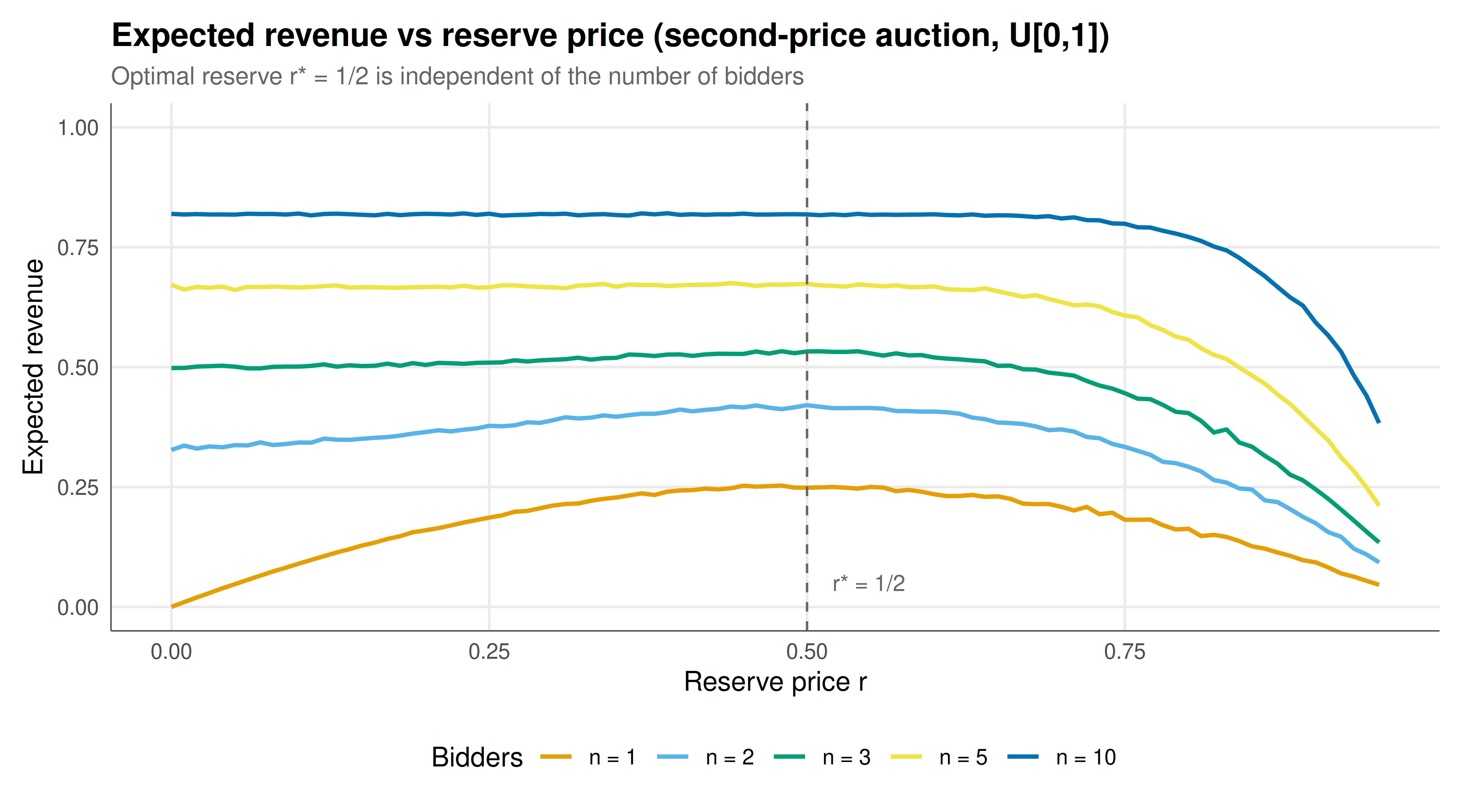
#| fig-cap: "Figure 1. Expected revenue as a function of reserve price in a second-price auction with uniform values on [0,1]. Each curve corresponds to a different number of bidders (n=1,2,3,5,10). The dashed vertical line marks the optimal reserve r*=1/2, which maximises revenue regardless of n. With few bidders, the reserve price has a large impact on revenue; with many bidders, competition alone drives revenue close to 1, and the reserve provides only a marginal improvement. Okabe-Ito palette."
#| dev: [png, pdf]
#| fig-width: 9
#| fig-height: 5
#| dpi: 300
reserve_seq <- seq(0, 0.95, by = 0.01)
n_values <- c(1, 2, 3, 5, 10)

rev_data <- expand.grid(reserve = reserve_seq, n_bidders = n_values) |>
  as_tibble() |>
  rowwise() |>
  mutate(revenue = simulate_revenue(n_bidders, reserve, n_sims = 10000)) |>
  ungroup() |>
  mutate(n_label = paste0("n = ", n_bidders),
         n_label = factor(n_label, levels = paste0("n = ", n_values)))

p_static <- ggplot(rev_data, aes(x = reserve, y = revenue, color = n_label)) +
  geom_line(linewidth = 0.9) +
  geom_vline(xintercept = 0.5, linetype = "dashed", color = "grey40", linewidth = 0.5) +
  annotate("text", x = 0.52, y = 0.05, label = "r* = 1/2", hjust = 0,
           color = "grey40", size = 3.5) +
  scale_color_manual(values = okabe_ito[1:5], name = "Bidders") +
  labs(title = "Expected revenue vs reserve price (second-price auction, U[0,1])",
       subtitle = "Optimal reserve r* = 1/2 is independent of the number of bidders",
       x = "Reserve price r", y = "Expected revenue") +
  theme_publication() +
  coord_cartesian(ylim = c(0, 1))

p_static
```
## Interactive figure
```{r}
#| label: fig-revenue-interactive
rev_data_interactive <- rev_data |>
  mutate(text = paste0("Reserve: ", round(reserve, 2),
                       "\nBidders: ", n_bidders,
                       "\nE[Revenue]: ", round(revenue, 4)))

p_int <- ggplot(rev_data_interactive,
                aes(x = reserve, y = revenue, color = n_label, text = text)) +
  geom_line(linewidth = 0.8) +
  geom_vline(xintercept = 0.5, linetype = "dashed", color = "grey40") +
  scale_color_manual(values = okabe_ito[1:5], name = "Bidders") +
  labs(title = "Expected revenue vs reserve price",
       subtitle = "Hover for details; dashed line = optimal reserve",
       x = "Reserve price r", y = "Expected revenue") +
  theme_publication()

ggplotly(p_int, tooltip = "text") |>
  config(displaylogo = FALSE, modeBarButtonsToRemove = c("select2d", "lasso2d"))
```
## Interpretation
The simulations confirm Myerson's theoretical prediction: for uniformly distributed values on $[0,1]$, the optimal reserve price is $r^* = 1/2$ regardless of the number of bidders. The economic intuition runs as follows. A reserve price is essentially a take-it-or-leave-it offer to a single bidder. When there is only one bidder ($n = 1$), the auction reduces to monopoly pricing, and the optimal price is $1/2$ (the monopoly price for a linear demand curve). When there are multiple bidders, competition raises the expected payment above $r^*$ in most realisations, so the reserve only binds in the marginal case where exactly one bidder values the object above $r$. The probability of this event shrinks with $n$, but the optimal threshold remains $1/2$ because the virtual valuation function --- and hence the point where it crosses zero --- depends only on the distribution, not on $n$. The revenue gains from an optimal reserve are most dramatic with few bidders (25% improvement for $n = 2$, over 100% for $n = 1$) and diminish as $n$ grows, since competition itself drives revenue toward the upper bound of the value distribution. For non-uniform distributions, the optimal reserve shifts: concave distributions (values concentrated near 1) have lower optimal reserves, while convex distributions (values concentrated near 0) have higher ones. This analysis assumes risk-neutral bidders and independent private values; with correlated values or risk-averse bidders, the optimal mechanism may involve different instruments beyond a simple reserve price.
## Extensions & related tutorials
- [First-price sealed-bid auction](../../auction-theory-deep-dive/first-price-sealed-bid/) --- equilibrium bidding in first-price auctions where reserve prices alter the strategy.
- [Vickrey auction and dominant-strategy incentive compatibility](../../mechanism-design/vickrey-second-price-auction/) --- the theoretical foundation for truthful second-price auctions.
- [Bayesian games under incomplete information](../bayesian-games-incomplete-information/) --- the general framework for games with private types.
- [Revenue equivalence theorem](../../auction-theory-deep-dive/revenue-equivalence-theorem/) --- why all standard auctions yield the same expected revenue.
- [Spectrum auction design (case study)](../../case-studies/spectrum-auction-design/) --- real-world application of auction design with reserve prices.
## References
::: {#refs}
:::