First-price sealed-bid auction — equilibrium bidding strategies

Derive the Bayesian Nash equilibrium of the first-price sealed-bid auction in R, show bid-shading as a function of the number of bidders, and compare revenue across auction formats.

Keywords

first-price auction, sealed-bid, bid shading, Bayesian Nash equilibrium, auction theory

Introduction & motivation

In a first-price sealed-bid auction, bidders submit sealed bids and the highest bidder wins, paying their own bid. Unlike the Vickrey auction where truthful bidding is dominant, first-price auctions create a strategic tension: bidding your true value guarantees zero surplus if you win, so rational bidders shade their bids below their values. The equilibrium amount of shading depends on the number of bidders and the distribution of values — more competition means less shading, as the risk of losing increases. The first-price auction is the most common auction format in practice: government procurement, construction contracts, oil lease sales, and many online auctions use first-price rules. Understanding the equilibrium bidding strategy is essential for auction design, bidder strategy, and revenue prediction. This tutorial derives the symmetric Bayesian Nash equilibrium for the independent private values model with uniform distributions, implements the equilibrium and simulates thousands of auctions, and visualizes how bid shading decreases with competition — ultimately confirming the revenue equivalence theorem that links first-price and second-price auctions.

Mathematical formulation

With \(n\) bidders and values \(v_i \sim U[0,1]\) independently, the symmetric BNE bidding strategy in the first-price auction is:

\[b^*(v) = \frac{n-1}{n} v\]

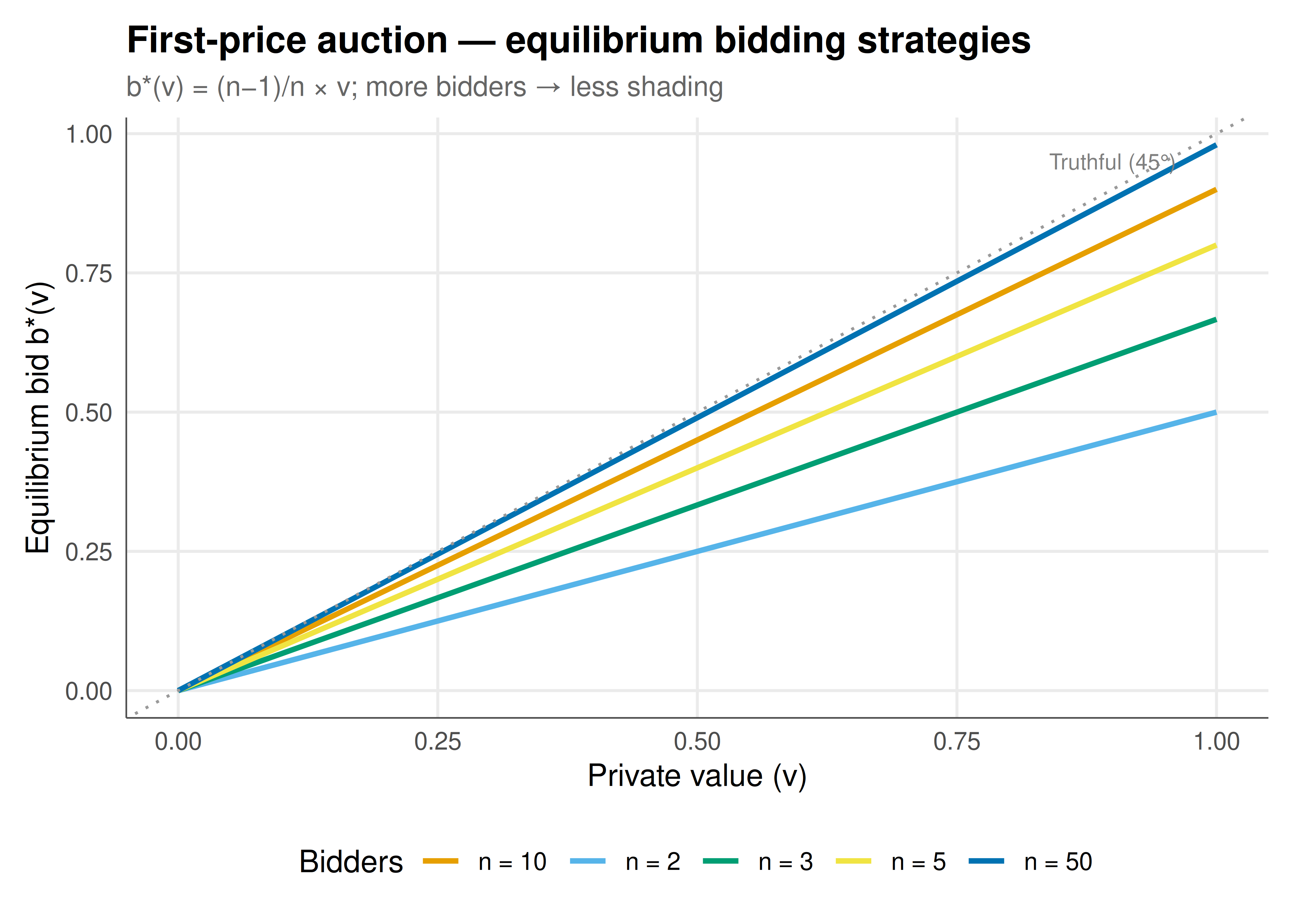
Derivation: Bidder \(i\) with value \(v\) bids \(b\) to maximise expected surplus \((v - b) \cdot P(\text{win})\). In a symmetric equilibrium where others use \(\beta(v) = \frac{n-1}{n}v\), bidder \(i\) wins when \(b > \beta(v_j)\) for all \(j \neq i\), i.e., \(v_j < \frac{nb}{n-1}\) for all opponents. Since values are \(U[0,1]\): \(P(\text{win}) = \left(\frac{nb}{n-1}\right)^{n-1}\). Maximising \((v-b)\left(\frac{nb}{n-1}\right)^{n-1}\) yields \(b^*(v) = \frac{n-1}{n}v\).

The bid shading factor \(1/n\) shrinks with competition: with 2 bidders, shade 50%; with 10, shade only 10%.

R implementation

bid_equilibrium <- function(v, n) (n - 1) / n * v

set.seed(42)
n_sims <- 10000

simulate_fpa <- function(n_bidders, n_sims) {
  revenues <- numeric(n_sims)
  winner_surpluses <- numeric(n_sims)
  for (s in 1:n_sims) {
    values <- runif(n_bidders)
    bids <- bid_equilibrium(values, n_bidders)
    winner <- which.max(bids)
    revenues[s] <- bids[winner]
    winner_surpluses[s] <- values[winner] - bids[winner]
  }
  tibble(n = n_bidders, revenue = revenues, surplus = winner_surpluses)
}

results <- lapply(c(2, 3, 5, 10, 20), simulate_fpa, n_sims = n_sims) |> bind_rows()

cat("=== First-Price Auction: Equilibrium Revenue by Number of Bidders ===\n")

=== First-Price Auction: Equilibrium Revenue by Number of Bidders ===

results |> group_by(n) |>
  summarise(mean_rev = mean(revenue), sd_rev = sd(revenue),
            mean_surplus = mean(surplus),
            theoretical = (n[1]-1)/(n[1]+1), .groups = "drop") |>
  mutate(across(where(is.numeric), ~round(., 4))) |> print()

# A tibble: 5 × 5
      n mean_rev sd_rev mean_surplus theoretical
  <dbl>    <dbl>  <dbl>        <dbl>       <dbl>
1     2    0.332 0.118        0.332        0.333
2     3    0.502 0.130        0.251        0.5  
3     5    0.667 0.113        0.167        0.667
4    10    0.818 0.0747       0.0909       0.818
5    20    0.905 0.042        0.0476       0.905

Static publication-ready figure

v_seq <- seq(0, 1, 0.01)
bid_df <- expand.grid(v = v_seq, n = c(2, 3, 5, 10, 50)) |>
  mutate(bid = bid_equilibrium(v, n), n_label = paste0("n = ", n))
ggplot(bid_df, aes(x = v, y = bid, color = n_label)) +
  geom_line(linewidth = 1) +
  geom_abline(slope = 1, intercept = 0, linetype = "dotted", color = "grey60") +
  scale_color_manual(values = okabe_ito[1:5], name = "Bidders") +
  annotate("text", x = 0.9, y = 0.95, label = "Truthful (45°)", size = 3, color = "grey50") +
  labs(title = "First-price auction — equilibrium bidding strategies",
       subtitle = "b*(v) = (n−1)/n × v; more bidders → less shading",
       x = "Private value (v)", y = "Equilibrium bid b*(v)") +
  theme_publication()

Figure 1: Figure 1. Equilibrium bidding strategies in the first-price auction for different numbers of bidders. With more competitors, bidders shade less (bid closer to their true value) because the probability of losing increases. In the limit of infinite bidders, bids converge to true values. Okabe-Ito palette.

Interactive figure

rev_summary <- results |> group_by(n) |>
  summarise(mean_rev = mean(revenue), sd_rev = sd(revenue),
            theoretical = (n[1]-1)/(n[1]+1), .groups = "drop") |>
  mutate(text = paste0("n = ", n, "\nMean revenue: ", round(mean_rev, 4),
                       "\nTheoretical: ", round(theoretical, 4)))
p_rev <- ggplot(rev_summary, aes(x = n, y = mean_rev, text = text)) +
  geom_line(color = okabe_ito[5], linewidth = 1) +
  geom_point(color = okabe_ito[5], size = 3) +
  geom_line(aes(y = theoretical), color = okabe_ito[3], linetype = "dashed", linewidth = 0.8) +
  labs(title = "Expected revenue vs number of bidders",
       subtitle = "Solid = simulated; dashed = theoretical (n−1)/(n+1)",
       x = "Number of bidders", y = "Expected revenue") +
  theme_publication()
ggplotly(p_rev, tooltip = "text") |>
  config(displaylogo = FALSE, modeBarButtonsToRemove = c("select2d", "lasso2d"))

Figure 2

Interpretation

The first-price auction equilibrium reveals the fundamental trade-off in competitive bidding: bid too low and risk losing to a competitor; bid too high and win but sacrifice surplus. The equilibrium strategy \(b^*(v) = \frac{n-1}{n}v\) optimally balances these forces, with the shading factor \(1/n\) decreasing as competition intensifies. With 2 bidders, the winner keeps half their surplus; with 20, they keep only 5%. The simulation confirms that expected revenue matches the theoretical prediction \((n-1)/(n+1)\) and equals the second-price auction’s revenue — validating the revenue equivalence theorem. This equivalence is remarkable: despite radically different strategic incentives (truthful vs shaded bidding), the expected payment to the seller is identical. In practice, first-price auctions may differ from second-price due to risk aversion (which increases bidding and revenue in first-price), asymmetric bidders, or collusion (easier in second-price). These deviations from the IPV model drive much of modern auction theory and design.

Extensions & related tutorials

• Vickrey second-price auction — the truthful counterpart.
• Zero-sum games and minimax — competitive optimization.
• Revenue equivalence theorem — formal proof and extensions.
• Common value auctions and the winner’s curse — when values are correlated.
• Google’s GSP auction — multi-unit extension for ad markets.

References