---
title: "Zero-sum games and the minimax theorem"
description: "Prove and implement von Neumann's minimax theorem for two-player zero-sum games in R, compute minimax strategies via linear programming, and visualize the security level geometry."
author: "Raban Heller"
date: 2026-05-08
date-modified: 2026-05-08
categories:
- foundations
- zero-sum
- minimax
- linear-programming
keywords: ["zero-sum game", "minimax theorem", "von Neumann", "saddle point", "linear programming", "security level"]
labels: ["equilibrium-concepts", "classical-results"]
tier: 1
bibliography: ../../../references.bib
vgwort: "TODO_VGWORT_foundations_zero-sum-minimax-theorem"
image: thumbnail.png
image-alt: "3D surface showing the minimax saddle point of a zero-sum game"
citation:
type: webpage
url: https://r-heller.github.io/equilibria/tutorials/foundations/zero-sum-minimax-theorem/
license: "CC BY-SA 4.0"
draft: false
has_static_fig: true
has_interactive_fig: true
has_shiny_app: false
---
```{r}
#| label: setup
#| include: false
library(ggplot2)
library(dplyr)
library(tidyr)
library(plotly)
library(lpSolve)
okabe_ito <- c("#E69F00", "#56B4E9", "#009E73", "#F0E442",
"#0072B2", "#D55E00", "#CC79A7", "#999999")
theme_publication <- function(base_size = 12) {
theme_minimal(base_size = base_size) +
theme(
plot.title = element_text(size = base_size * 1.2, face = "bold"),
plot.subtitle = element_text(size = base_size * 0.9, color = "grey40"),
axis.line = element_line(color = "grey30", linewidth = 0.3),
panel.grid.minor = element_blank(),
legend.position = "bottom",
plot.margin = margin(10, 10, 10, 10)
)
}
```
## Introduction & motivation
The minimax theorem, proved by John @von_neumann_morgenstern_1944 in 1928 (predating the comprehensive 1944 book), is the foundational result of game theory. It states that in any finite two-player zero-sum game, there exists a value $v$ such that the row player can guarantee an expected payoff of at least $v$ (the maximin value) and the column player can guarantee that the row player receives at most $v$ (the minimax value). The fact that these two values are equal — $\max_p \min_q p^\top A q = \min_q \max_p p^\top A q = v$ — is profound: it means the game has a determinate value, and neither player can do better by being smarter than the other if both play optimally. The minimax theorem predates Nash's equilibrium concept by over two decades and remains the cleanest, most elegant result in game theory. It also connects game theory to linear programming: computing minimax strategies for zero-sum games is equivalent to solving a pair of dual linear programs. This tutorial implements minimax strategy computation for arbitrary $m \times n$ zero-sum games using both direct enumeration (for small games) and linear programming (for larger games), and visualizes the geometry of the minimax saddle point.
## Mathematical formulation
In a two-player zero-sum game, the payoff matrix $A$ gives the row player's payoffs; the column player's payoffs are $-A$. Let $p \in \Delta^m$ be the row player's mixed strategy and $q \in \Delta^n$ be the column player's mixed strategy, where $\Delta^k$ denotes the probability simplex.
The **minimax theorem** states:
$$
\max_{p \in \Delta^m} \min_{q \in \Delta^n} p^\top A q = \min_{q \in \Delta^n} \max_{p \in \Delta^m} p^\top A q = v
$$
The common value $v$ is the **value of the game**. A pair $(p^*, q^*)$ achieving this value is a **minimax equilibrium** (equivalently, a Nash equilibrium of the zero-sum game).
**Computing via LP**: The row player's problem is:
$$
\max \, v \quad \text{s.t.} \quad p^\top A e_j \geq v \;\; \forall j, \quad p \in \Delta^m
$$
which is a linear program. The column player's problem is its dual.
## R implementation
```{r}
#| label: minimax-solver
# Minimax solver using linear programming
solve_minimax <- function(A) {
  m <- nrow(A)
  n <- ncol(A)

  # Shift payoffs to ensure positivity (LP trick)
  shift <- max(0, -min(A)) + 1
  A_pos <- A + shift

  # Row player LP: maximise game value v
  # Variables: p_1, ..., p_m, v
  # max v  s.t.  sum_i p_i * A[i,j] >= v for all j,  sum p_i = 1, p_i >= 0
  # Equivalently: let y_i = p_i / v, maximise 1/v = sum y_i
  # This is the standard LP formulation

  # Using lpSolve: minimize -v subject to Ap >= v*1, sum(p) = 1
  # Reformulate: let z_i = p_i; maximize v
  # A^T z >= v * 1_n, sum(z) = 1, z >= 0

  f.obj <- c(rep(0, m), 1)  # maximize v (last variable)
  f.con <- rbind(
    cbind(t(A_pos), -rep(1, n)),  # A^T p >= v (one row per col strategy)
    c(rep(1, m), 0)               # sum(p) = 1
  )
  f.dir <- c(rep(">=", n), "=")
  f.rhs <- c(rep(0, n), 1)

  sol <- lp("max", f.obj, f.con, f.dir, f.rhs)

  p_star <- sol$solution[1:m]
  game_value <- sol$objval - shift

  # Column player (dual): minimize w s.t. Aq <= w*1, sum(q) = 1
  f.obj2 <- c(rep(0, n), 1)
  f.con2 <- rbind(
    cbind(A_pos, -rep(1, m)),
    c(rep(1, n), 0)
  )
  f.dir2 <- c(rep("<=", m), "=")
  f.rhs2 <- c(rep(0, m), 1)

  sol2 <- lp("min", f.obj2, f.con2, f.dir2, f.rhs2)
  q_star <- sol2$solution[1:n]

  list(p = p_star, q = q_star, value = game_value)
}

# --- Example 1: Matching Pennies ---
cat("=== Matching Pennies ===\n")
A_mp <- matrix(c(1, -1, -1, 1), nrow = 2,
               dimnames = list(c("H","T"), c("H","T")))
print(A_mp)
mp_result <- solve_minimax(A_mp)
cat(sprintf("Value: %.2f\nRow strategy: (%.3f, %.3f)\nCol strategy: (%.3f, %.3f)\n\n",
            mp_result$value, mp_result$p[1], mp_result$p[2],
            mp_result$q[1], mp_result$q[2]))
# --- Example 2: 3x3 game ---
cat("=== 3×3 Zero-Sum Game ===\n")
A3 <- matrix(c(3, -1, 2,
               -2, 4, -3,
               1, 0, 1), nrow = 3, byrow = TRUE,
             dimnames = list(paste0("R",1:3), paste0("C",1:3)))
print(A3)
result3 <- solve_minimax(A3)
cat(sprintf("Value: %.3f\nRow strategy: (%s)\nCol strategy: (%s)\n",
            result3$value,
            paste(round(result3$p, 3), collapse = ", "),
            paste(round(result3$q, 3), collapse = ", ")))
```
## Static publication-ready figure
```{r}
#| label: fig-minimax-geometry
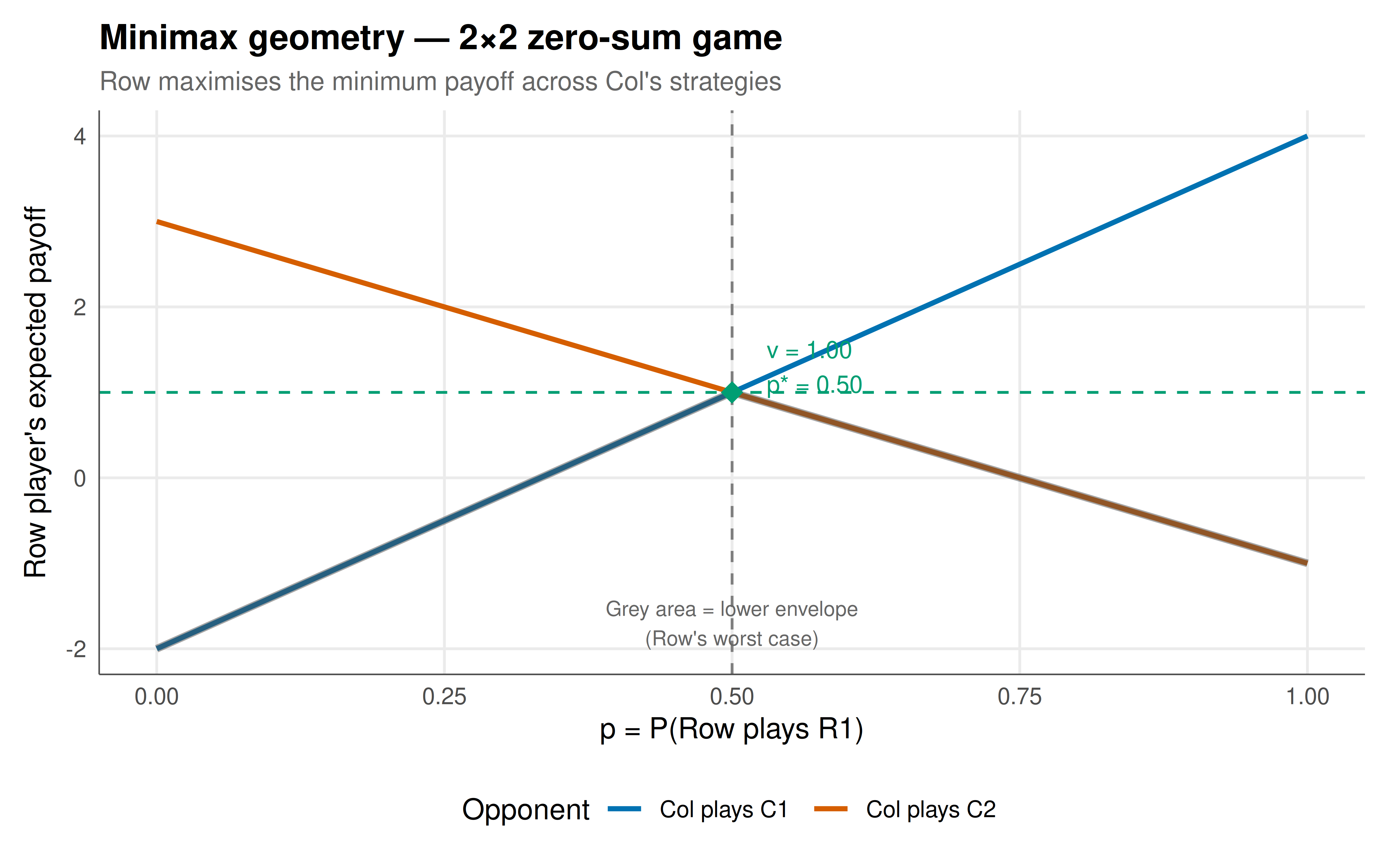
#| fig-cap: "Figure 1. Minimax geometry for a 2×2 zero-sum game. The row player's expected payoff is plotted as a function of the mixing probability p for each of the column player's pure strategies. The lower envelope (worst case for Row) is maximised at the intersection — this is the minimax strategy. The game value (dashed line) is where the maximin and minimax meet. Okabe-Ito palette."
#| dev: [png, pdf]
#| fig-width: 8
#| fig-height: 5
#| dpi: 300
# Visualise for a 2x2 game with asymmetric payoffs
A_vis <- matrix(c(4, -2, -1, 3), nrow = 2)

p_seq <- seq(0, 1, by = 0.005)

payoff_data <- tibble(p = p_seq) |>
  mutate(
    vs_C1 = p * A_vis[1,1] + (1-p) * A_vis[2,1],
    vs_C2 = p * A_vis[1,2] + (1-p) * A_vis[2,2],
    min_payoff = pmin(vs_C1, vs_C2)
  )

# Find optimal p
opt_p <- p_seq[which.max(payoff_data$min_payoff)]
game_val <- max(payoff_data$min_payoff)

payoff_long <- payoff_data |>
  select(p, vs_C1, vs_C2) |>
  pivot_longer(-p, names_to = "opponent", values_to = "payoff") |>
  mutate(opponent = ifelse(opponent == "vs_C1", "Col plays C1", "Col plays C2"))

p_geom <- ggplot() +
  geom_line(data = payoff_long, aes(x = p, y = payoff, color = opponent),
            linewidth = 1) +
  geom_line(data = payoff_data, aes(x = p, y = min_payoff),
            linewidth = 1.5, color = "grey30", alpha = 0.5) +
  geom_vline(xintercept = opt_p, linetype = "dashed", color = "grey50") +
  geom_hline(yintercept = game_val, linetype = "dashed", color = okabe_ito[3]) +
  geom_point(aes(x = opt_p, y = game_val), color = okabe_ito[3], size = 4, shape = 18) +
  annotate("text", x = opt_p + 0.03, y = game_val + 0.3,
           label = sprintf("v = %.2f\np* = %.2f", game_val, opt_p),
           size = 3.5, hjust = 0, color = okabe_ito[3]) +
  annotate("text", x = 0.5, y = min(payoff_long$payoff) + 0.3,
           label = "Grey area = lower envelope\n(Row's worst case)",
           size = 3, color = "grey40") +
  scale_color_manual(values = c(okabe_ito[5], okabe_ito[6]), name = "Opponent") +
  labs(
    title = "Minimax geometry — 2×2 zero-sum game",
    subtitle = "Row maximises the minimum payoff across Col's strategies",
    x = "p = P(Row plays R1)", y = "Row player's expected payoff"
  ) +
  theme_publication()

p_geom
```
## Interactive figure
```{r}
#| label: fig-minimax-3x3-interactive
# Visualise the 3x3 game's payoff landscape
A3_vis <- A3
p1_seq <- seq(0, 1, by = 0.02)

# Row player with 3 strategies: p1, p2, 1-p1-p2
grid3 <- expand.grid(p1 = p1_seq, p2 = p1_seq) |>
  filter(p1 + p2 <= 1) |>
  mutate(p3 = 1 - p1 - p2)

# Expected payoff against each column strategy
grid3$vs_C1 <- grid3$p1 * A3_vis[1,1] + grid3$p2 * A3_vis[2,1] + grid3$p3 * A3_vis[3,1]
grid3$vs_C2 <- grid3$p1 * A3_vis[1,2] + grid3$p2 * A3_vis[2,2] + grid3$p3 * A3_vis[3,2]
grid3$vs_C3 <- grid3$p1 * A3_vis[1,3] + grid3$p2 * A3_vis[2,3] + grid3$p3 * A3_vis[3,3]
grid3$min_payoff <- pmin(grid3$vs_C1, grid3$vs_C2, grid3$vs_C3)

grid3_text <- grid3 |>
  mutate(text = paste0("p = (", round(p1,2), ", ", round(p2,2), ", ", round(p3,2), ")",
                       "\nMin payoff: ", round(min_payoff, 2)))

# Barycentric to Cartesian
grid3_text <- grid3_text |>
  mutate(cx = p2 + 0.5 * p3,
         cy = (sqrt(3)/2) * p3)

p_3x3 <- ggplot(grid3_text, aes(x = cx, y = cy, fill = min_payoff, text = text)) +
  geom_tile(width = 0.015, height = 0.015) +
  scale_fill_gradient2(low = okabe_ito[6], mid = okabe_ito[4], high = okabe_ito[3],
                        midpoint = result3$value, name = "Min payoff") +
  annotate("text", x = 0, y = -0.04, label = "R1", size = 3) +
  annotate("text", x = 1, y = -0.04, label = "R2", size = 3) +
  annotate("text", x = 0.5, y = sqrt(3)/2 + 0.04, label = "R3", size = 3) +
  coord_fixed() +
  labs(
    title = "Minimax landscape on the strategy simplex (3×3 game)",
    subtitle = sprintf("Game value = %.3f; brighter = higher security level", result3$value)
  ) +
  theme_publication() +
  theme(axis.text = element_blank(), axis.title = element_blank(),
        axis.ticks = element_blank(), axis.line = element_blank(),
        panel.grid = element_blank())

ggplotly(p_3x3, tooltip = "text") |>
  config(displaylogo = FALSE,
         modeBarButtonsToRemove = c("select2d", "lasso2d"))
```
## Interpretation
The minimax theorem's power lies in its guarantee: in any zero-sum game, there is a strategy that is **simultaneously optimal** against the worst case and optimal in equilibrium. The 2×2 geometric visualization makes this concrete — the row player's minimax strategy is the mixing probability that maximises the lower envelope of their payoff lines, and this maximum exactly equals the game value. For the 3×3 game, the strategy simplex heatmap shows that the minimax strategy sits at a uniquely bright peak of the security-level landscape. The LP solver handles arbitrary game sizes efficiently (polynomial in the number of strategies), making minimax computation practical even for large zero-sum games. The historical significance of this result cannot be overstated: @von_neumann_morgenstern_1944 proved it using Brouwer's fixed-point theorem (a topological argument), and it inspired both Nash's generalisation to non-zero-sum games and the development of linear programming by Dantzig. In practical applications, minimax strategies appear in competitive settings ranging from poker (where GTO play is a minimax strategy) to adversarial machine learning (where robustness against worst-case perturbations is a minimax problem) to military strategy (where ensuring a minimal guaranteed outcome is a security-first approach).
## Extensions & related tutorials
- [Mixed-strategy Nash equilibrium in 2×2 games](../nash-equilibrium-mixed/) — generalising beyond zero-sum.
- [Dominant strategies and IESDS](../dominant-strategies-iterated-elimination/) — when dominance solves the game.
- [Linear programming for game theory](../../optimization-numerical-methods/lp-game-theory/) — the LP duality connection in depth.
- [Poker GTO strategies](../../classical-games/poker-gto/) — minimax applied to imperfect information games.
- [Adversarial robustness in ML](../../ai-ml-foundations-and-applications/adversarial-robustness/) — minimax in machine learning.
## References
::: {#refs}
:::