Mixed-strategy Nash equilibrium in 2×2 games

How to compute a mixed-strategy Nash equilibrium for a 2×2 normal-form game, with R and Python implementations and interactive visualizations.

Keywords

nash equilibrium, mixed strategies, indifference principle, best response, R, nashpy

Introduction & motivation

Many games have no equilibrium in pure strategies. Consider Matching Pennies: one player wants the coins to match, the other wants them to differ. Whatever pure strategy a player picks, the opponent can exploit it. The resolution, due to Nash (1950), is to allow players to randomize — choosing each action with some probability. A mixed-strategy Nash equilibrium is a profile of probability distributions, one per player, such that no player can increase their expected payoff by unilaterally changing their distribution. In a finite 2×2 game the mixed equilibrium is found by the indifference principle: each player’s mixture must make the opponent indifferent between their own pure strategies. This article derives the indifference conditions, implements the computation in R and Python, and visualizes the best-response correspondences whose intersection pins down the equilibrium. Mixed equilibria are central to applications ranging from penalty kicks in football to randomized auditing in tax compliance, and understanding them is a prerequisite for nearly everything else in non-cooperative game theory.

Mathematical formulation

Consider a 2×2 game with payoff matrices for the row player (Player 1) and column player (Player 2):

\[ A = \begin{pmatrix} a_{11} & a_{12} \\ a_{21} & a_{22} \end{pmatrix}, \quad B = \begin{pmatrix} b_{11} & b_{12} \\ b_{21} & b_{22} \end{pmatrix} \]

Player 1 chooses row \(T\) (top) with probability \(p\) and row \(B\) (bottom) with probability \(1-p\). Player 2 chooses column \(L\) with probability \(q\) and column \(R\) with probability \(1-q\). At a mixed-strategy Nash equilibrium, each player must be indifferent between their pure strategies given the opponent’s mixture. The indifference condition for Player 2 (making Player 1 indifferent) is:

\[ q \cdot a_{11} + (1-q) \cdot a_{12} = q \cdot a_{21} + (1-q) \cdot a_{22} \]

Solving for \(q\):

\[ q^* = \frac{a_{22} - a_{12}}{a_{11} - a_{12} - a_{21} + a_{22}} \]

Symmetrically, the indifference condition for Player 1 (making Player 2 indifferent) gives:

\[ p^* = \frac{b_{22} - b_{21}}{b_{11} - b_{21} - b_{12} + b_{22}} \]

A mixed-strategy Nash equilibrium \((p^*, q^*)\) exists whenever \(0 \le p^* \le 1\) and \(0 \le q^* \le 1\) and no pure-strategy equilibrium already makes the indifference conditions vacuous. Nash (1951) proved that every finite game has at least one Nash equilibrium, which may be in mixed strategies. Harsanyi (1973) provided a deeper justification: mixed equilibria arise as limits of pure-strategy equilibria in nearby games with slightly perturbed payoffs, so randomization reflects genuine uncertainty rather than literal coin-flipping.

R implementation

The function below computes all Nash equilibria — pure and mixed — for any 2×2 game specified by its payoff matrices \(A\) (row player) and \(B\) (column player). It checks for pure-strategy equilibria via best-response comparisons, then applies the indifference principle for the mixed equilibrium.

nash_2x2 <- function(A, B) {
  equilibria <- list()

  # --- Pure-strategy Nash equilibria ---
  # (i,j) is a PSNE if a[i,j] >= a[k,j] for all k and b[i,j] >= b[i,l] for all l
  for (i in 1:2) {
    for (j in 1:2) {
      row_best <- A[i, j] >= A[3 - i, j]
      col_best <- B[i, j] >= B[i, 3 - j]
      if (row_best && col_best) {
        equilibria <- c(equilibria, list(list(
          type = "pure",
          p = ifelse(i == 1, 1, 0),
          q = ifelse(j == 1, 1, 0),
          label = paste0("Pure: (", c("T","B")[i], ", ", c("L","R")[j], ")")
        )))
      }
    }
  }

  # --- Mixed-strategy Nash equilibrium ---
  denom_q <- A[1,1] - A[1,2] - A[2,1] + A[2,2]
  denom_p <- B[1,1] - B[2,1] - B[1,2] + B[2,2]

  if (abs(denom_q) > 1e-12 && abs(denom_p) > 1e-12) {
    q_star <- (A[2,2] - A[1,2]) / denom_q
    p_star <- (B[2,2] - B[2,1]) / denom_p

    if (q_star > 0 && q_star < 1 && p_star > 0 && p_star < 1) {
      # Expected payoffs at equilibrium
      eu1 <- p_star * (q_star * A[1,1] + (1 - q_star) * A[1,2]) +
             (1 - p_star) * (q_star * A[2,1] + (1 - q_star) * A[2,2])
      eu2 <- p_star * (q_star * B[1,1] + (1 - q_star) * B[1,2]) +
             (1 - p_star) * (q_star * B[2,1] + (1 - q_star) * B[2,2])

      equilibria <- c(equilibria, list(list(
        type  = "mixed",
        p     = round(p_star, 4),
        q     = round(q_star, 4),
        eu1   = round(eu1, 4),
        eu2   = round(eu2, 4),
        label = sprintf("Mixed: p*=%.4f, q*=%.4f", p_star, q_star)
      )))
    }
  }

  equilibria
}

# --- Example: Matching Pennies ---
A_mp <- matrix(c(1, -1, -1, 1), nrow = 2, byrow = TRUE)
B_mp <- matrix(c(-1, 1, 1, -1), nrow = 2, byrow = TRUE)

cat("Matching Pennies:\n")

Matching Pennies:

cat("  A =", A_mp[1,], "/", A_mp[2,], "\n")

  A = 1 -1 / -1 1 

cat("  B =", B_mp[1,], "/", B_mp[2,], "\n\n")

  B = -1 1 / 1 -1 

eqs <- nash_2x2(A_mp, B_mp)
for (eq in eqs) {
  cat(" ", eq$label, "\n")
  if (eq$type == "mixed") cat("    EU1 =", eq$eu1, ", EU2 =", eq$eu2, "\n")
}

  Mixed: p*=0.5000, q*=0.5000 
    EU1 = 0 , EU2 = 0 

# --- Example: Battle of the Sexes ---
A_bos <- matrix(c(3, 0, 0, 2), nrow = 2, byrow = TRUE)
B_bos <- matrix(c(2, 0, 0, 3), nrow = 2, byrow = TRUE)

cat("\nBattle of the Sexes:\n")

Battle of the Sexes:

eqs_bos <- nash_2x2(A_bos, B_bos)
for (eq in eqs_bos) {
  cat(" ", eq$label, "\n")
  if (eq$type == "mixed") cat("    EU1 =", eq$eu1, ", EU2 =", eq$eu2, "\n")
}

  Pure: (T, L) 
  Pure: (B, R) 
  Mixed: p*=0.6000, q*=0.4000 
    EU1 = 1.2 , EU2 = 1.2 

Static publication-ready figure

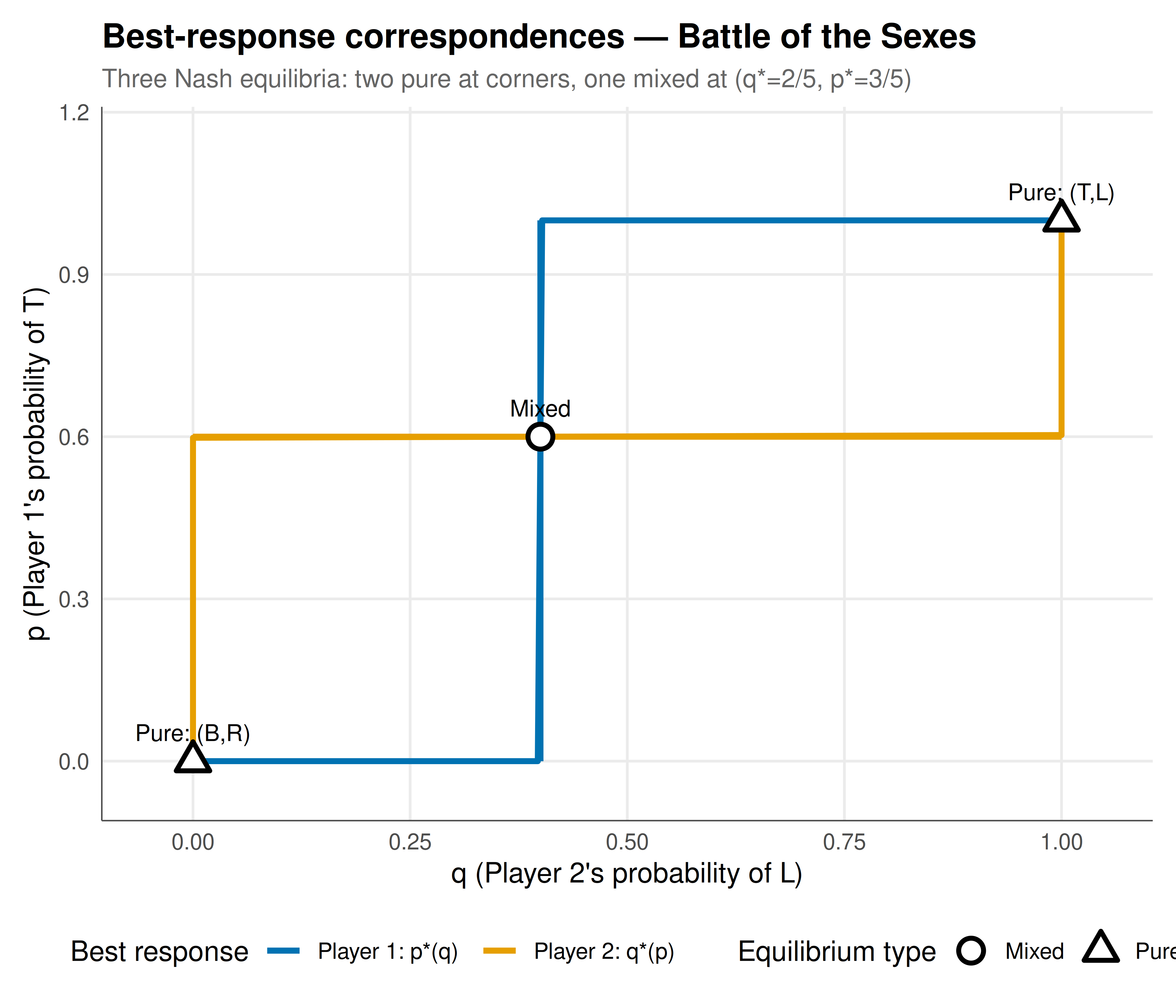
The best-response correspondences show each player’s optimal probability as a function of the opponent’s mixture. The intersection of these correspondences is the Nash equilibrium. Below we plot this for the Battle of the Sexes game, where the two pure equilibria appear at the corners and the mixed equilibrium sits where the curves cross.

# Battle of the Sexes payoffs
A <- matrix(c(3, 0, 0, 2), nrow = 2, byrow = TRUE)
B <- matrix(c(2, 0, 0, 3), nrow = 2, byrow = TRUE)

# Best response for Player 1: given q, choose p to maximize expected payoff
# EU1(T) = 3q, EU1(B) = 2(1-q) => BR1: p=1 if 3q > 2-2q => q > 2/5
# At q = 2/5, Player 1 is indifferent
q_grid <- seq(0, 1, length.out = 200)
br1_p <- ifelse(q_grid < 2/5, 0, ifelse(q_grid > 2/5, 1, NA))

# Best response for Player 2: given p, choose q to maximize
# EU2(L) = 2p, EU2(R) = 3(1-p) => BR2: q=1 if 2p > 3-3p => p > 3/5
p_grid <- seq(0, 1, length.out = 200)
br2_q <- ifelse(p_grid < 3/5, 0, ifelse(p_grid > 3/5, 1, NA))

# Build data frames for plotting
df_br1 <- data.frame(q = q_grid, p = br1_p, player = "Player 1: p*(q)")
df_br2 <- data.frame(q = br2_q, p = p_grid, player = "Player 2: q*(p)")

# Indifference segments (vertical/horizontal at threshold)
df_indiff1 <- data.frame(q = c(2/5, 2/5), p = c(0, 1), player = "Player 1: p*(q)")
df_indiff2 <- data.frame(q = c(0, 1), p = c(3/5, 3/5), player = "Player 2: q*(p)")

# Equilibrium points
eq_pts <- data.frame(
  q = c(0, 1, 2/5),
  p = c(0, 1, 3/5),
  label = c("Pure: (B,R)", "Pure: (T,L)", "Mixed"),
  type = c("Pure", "Pure", "Mixed")
)

p_fig <- ggplot() +
  # BR correspondences as step functions
  geom_line(data = df_br1 |> filter(!is.na(p)),
            aes(x = q, y = p, color = player), linewidth = 1.2) +
  geom_segment(data = df_indiff1,
               aes(x = q[1], xend = q[2], y = p[1], yend = p[2], color = player),
               linewidth = 1.2, linetype = "solid") +
  geom_line(data = df_br2 |> filter(!is.na(q)),
            aes(x = q, y = p, color = player), linewidth = 1.2) +
  geom_segment(data = df_indiff2,
               aes(x = q[1], xend = q[2], y = p[1], yend = p[2], color = player),
               linewidth = 1.2, linetype = "solid") +
  # Equilibrium points
  geom_point(data = eq_pts, aes(x = q, y = p, shape = type),
             size = 4, fill = "white", stroke = 1.5) +
  geom_text(data = eq_pts, aes(x = q, y = p, label = label),
            vjust = -1.2, size = 3.5) +
  scale_color_manual(values = c(okabe_ito[5], okabe_ito[1])) +
  scale_shape_manual(values = c(Mixed = 21, Pure = 24)) +
  labs(
    title = "Best-response correspondences — Battle of the Sexes",
    subtitle = "Three Nash equilibria: two pure at corners, one mixed at (q*=2/5, p*=3/5)",
    x = "q (Player 2's probability of L)",
    y = "p (Player 1's probability of T)",
    color = "Best response",
    shape = "Equilibrium type"
  ) +
  coord_cartesian(xlim = c(-0.05, 1.05), ylim = c(-0.05, 1.15)) +
  theme_publication()

p_fig

Figure 1: Figure 1. Best-response correspondences for Battle of the Sexes. The blue curve is Player 1’s best response p(q); the orange curve is Player 2’s best response q(p). Dots mark the three Nash equilibria: two pure (corners) and one mixed (interior crossing). Okabe-Ito palette.

Interactive figure

The interactive version lets you hover over the best-response curves to read exact probability values and expected payoffs at each point.

# Compute expected payoffs along the BR curves for tooltips
br_data <- bind_rows(
  tibble(
    q = seq(0, 2/5 - 0.001, length.out = 50),
    p = 0,
    player = "Player 1",
    text = sprintf("q=%.3f, BR: p=0 (play B)\nEU1=%.3f", q, 2*(1-q))
  ),
  tibble(
    q = seq(2/5 + 0.001, 1, length.out = 50),
    p = 1,
    player = "Player 1",
    text = sprintf("q=%.3f, BR: p=1 (play T)\nEU1=%.3f", q, 3*q)
  ),
  tibble(
    p = seq(0, 3/5 - 0.001, length.out = 50),
    q = 0,
    player = "Player 2",
    text = sprintf("p=%.3f, BR: q=0 (play R)\nEU2=%.3f", p, 3*(1-p))
  ),
  tibble(
    p = seq(3/5 + 0.001, 1, length.out = 50),
    q = 1,
    player = "Player 2",
    text = sprintf("p=%.3f, BR: q=1 (play L)\nEU2=%.3f", p, 2*p)
  )
)

p_interactive <- ggplot(br_data, aes(x = q, y = p, color = player, text = text)) +
  geom_point(size = 0.8, alpha = 0.7) +
  # Indifference lines
  geom_segment(aes(x = 2/5, xend = 2/5, y = 0, yend = 1),
               color = okabe_ito[5], linewidth = 0.8, inherit.aes = FALSE) +
  geom_segment(aes(x = 0, xend = 1, y = 3/5, yend = 3/5),
               color = okabe_ito[1], linewidth = 0.8, inherit.aes = FALSE) +
  # Equilibria
  geom_point(data = eq_pts, aes(x = q, y = p), color = "black",
             size = 3, inherit.aes = FALSE) +
  scale_color_manual(values = c(okabe_ito[5], okabe_ito[1])) +
  labs(x = "q (P2 plays L)", y = "p (P1 plays T)", color = "Player") +
  theme_publication()

ggplotly(p_interactive, tooltip = "text") |>
  config(displaylogo = FALSE,
         modeBarButtonsToRemove = c("select2d", "lasso2d"))

Figure 2

Verification with Python’s nashpy

As a cross-check, we can verify our results using the nashpy library, which implements the support enumeration algorithm for finding all Nash equilibria of bimatrix games. This demonstrates the interoperability between R and Python that we use throughout #equilibria.

# Requires: pip install nashpy
library(reticulate)
nashpy <- import("nashpy")
np <- import("numpy")

# Battle of the Sexes
A <- np$array(matrix(c(3, 0, 0, 2), nrow = 2, byrow = TRUE))
B <- np$array(matrix(c(2, 0, 0, 3), nrow = 2, byrow = TRUE))
game <- nashpy$Game(A, B)

# Find all equilibria via support enumeration
eqs <- game$support_enumeration()
cat("nashpy equilibria for Battle of the Sexes:\n")
for (eq in iterate(eqs)) {
  cat(sprintf("  p = (%.4f, %.4f), q = (%.4f, %.4f)\n",
              eq[[1]][1], eq[[1]][2], eq[[2]][1], eq[[2]][2]))
}

Interpretation

The Battle of the Sexes has three Nash equilibria: two pure — (T, L) and (B, R) — and one mixed where Player 1 plays T with probability \(p^* = 3/5\) and Player 2 plays L with probability \(q^* = 2/5\). Several observations are worth emphasizing. First, the mixed equilibrium yields lower expected payoffs for both players (EU1 = 1.2, EU2 = 1.2) than either pure equilibrium (3,2) or (2,3). This is a general phenomenon: mixed equilibria in coordination games are often Pareto-dominated by pure ones, which raises the question of why players would randomize. Harsanyi (1973) provides the canonical answer: mixed equilibria are limits of pure equilibria in slightly perturbed games, so they reflect the players’ uncertainty about each other’s exact preferences rather than deliberate coin-flipping. Second, the indifference principle has a counter-intuitive implication: each player’s equilibrium mixture depends only on the opponent’s payoffs, not their own. Player 1’s randomization probability \(p^*\) is determined entirely by \(B\), because its purpose is to make Player 2 indifferent. Third, the best-response diagram makes the equilibrium structure visually transparent — the step-function correspondences can only intersect at corners (pure equilibria) or at the unique interior crossing (mixed equilibrium). This geometric insight extends directly to larger games via the Lemke-Howson algorithm (Lemke and Howson 1964), though computation becomes substantially harder beyond \(2 \times 2\).

Linked Shiny app

Open app in new tab · View source on GitHub

Extensions & related tutorials

This article covers the basic case. Several natural extensions and related concepts are explored elsewhere:

• Pure-strategy Nash equilibrium in 2×2 games — the simpler case where randomization is unnecessary.
• Best-response correspondences and equilibrium existence — the fixed-point argument behind Nash’s existence theorem.
• Correlated equilibrium (Aumann) — a generalization that allows coordination via public signals.
• The Lemke-Howson algorithm walked through — an algorithm for finding Nash equilibria in larger bimatrix games.
• Matching Pennies and mixed strategies — the canonical zero-sum example.

References

Harsanyi, John C. 1973. “Games with Randomly Disturbed Payoffs: A New Rationale for Mixed-Strategy Equilibrium Points.” International Journal of Game Theory 2 (1): 1–23. https://doi.org/10.1007/BF01737554.

Lemke, Carlton E., and Joseph T. Howson. 1964. “Equilibrium Points of Bimatrix Games.” Journal of the Society for Industrial and Applied Mathematics 12 (2): 413–23. https://doi.org/10.1137/0112033.

Nash, John F. 1950. “Equilibrium Points in n-Person Games.” Proceedings of the National Academy of Sciences 36 (1): 48–49. https://doi.org/10.1073/pnas.36.1.48.

Nash, John F. 1951. “Non-Cooperative Games.” Annals of Mathematics 54 (2): 286–95. https://doi.org/10.2307/1969529.