---
title: "Common-value auctions and the winner's curse"
description: "Derive, simulate, and visualize the winner's curse in common-value auctions: why naive bidding leads to systematic overpayment, and how rational bidders correct for the informational content of winning."
author: "Raban Heller"
date: 2026-05-08
date-modified: 2026-05-08
categories:
- auction-theory-deep-dive
- common-value-auctions
- winners-curse
- information-economics
keywords: ["winner's curse", "common value auction", "signal extraction", "conditional expectation", "oil lease auction"]
labels: ["auction-theory", "information-economics"]
tier: 1
bibliography: ../../../references.bib
vgwort: "TODO_VGWORT_auction-theory-deep-dive_common-value-winners-curse"
image: thumbnail.png
image-alt: "Expected profit comparison showing naive bidders suffering losses versus rational bidders earning positive profits in common-value auctions with varying numbers of bidders"
citation:
type: webpage
url: https://r-heller.github.io/equilibria/tutorials/auction-theory-deep-dive/common-value-winners-curse/
license: "CC BY-SA 4.0"
draft: false
has_static_fig: true
has_interactive_fig: true
has_shiny_app: false
---
```{r}
#| label: setup
#| include: false
library(ggplot2)
library(dplyr)
library(tidyr)
library(plotly)
okabe_ito <- c("#E69F00", "#56B4E9", "#009E73", "#F0E442",
"#0072B2", "#D55E00", "#CC79A7", "#999999")
theme_publication <- function(base_size = 12) {
theme_minimal(base_size = base_size) +
theme(plot.title = element_text(size = base_size * 1.2, face = "bold"),
plot.subtitle = element_text(size = base_size * 0.9, color = "grey40"),
axis.line = element_line(color = "grey30", linewidth = 0.3),
panel.grid.minor = element_blank(), legend.position = "bottom",
plot.margin = margin(10, 10, 10, 10))
}
```
## Introduction & motivation
In a private-value auction, each bidder knows exactly how much the item is worth to them. A painting enthusiast bidding on a Monet knows their own willingness to pay. But many real-world auctions involve **common values**: the item has the same intrinsic value to all bidders, but that value is unknown and each bidder has only a noisy estimate of it. The canonical example is an oil lease auction: the tract of land contains a fixed (but unknown) quantity of oil, and each firm has conducted its own geological survey yielding a noisy signal of the tract's value. Other examples include initial public offerings (the firm has one true value, but analysts disagree), takeover bids for companies, and procurement auctions where the true cost of a project is uncertain.
In common-value settings, a devastating phenomenon known as the **winner's curse** can trap inexperienced bidders. The logic is simple but subtle: if you win the auction, your signal must have been the highest among all bidders. But the highest signal from $n$ noisy estimates is likely an *overestimate* of the true value — it is the maximum order statistic of the signal distribution, which is biased upward. A naive bidder who bids their signal (or their unconditional estimate of value given their signal) will systematically overpay: conditional on winning, the expected true value is less than the winner's signal. This is not a matter of irrationality in some loose sense — it is a precise statistical phenomenon. The naive bidder fails to condition on the informational content of the event "I won," which is itself informative about the true value.
The winner's curse was first identified in the context of U.S. offshore oil lease auctions in the 1970s by Capen, Clapp, and Campbell (1971), who showed that oil companies were earning below-normal returns on their lease acquisitions. Rational bidders must account for the winner's curse by **shading their bids below their signal** — bidding not what they think the item is worth given their signal alone, but what they think it is worth given their signal *and the additional information that their signal is the highest*. This is the equilibrium bidding strategy in common-value auctions, first derived by Wilson (1977) for the first-price sealed-bid format. The magnitude of the correction depends critically on the number of bidders: with more bidders, the winner's signal is a more extreme order statistic, and the curse is more severe, requiring more aggressive bid shading.
In this tutorial, we implement a common-value auction model where the true value $V$ and bidder signals $S_i = V + \epsilon_i$ are normally distributed. We simulate both naive bidding (bid = signal) and rational equilibrium bidding (bid = $E[V | S_i = s_i, S_i = \max_j S_j]$), and we show that naive bidders suffer systematic losses while rational bidders earn positive expected profit. We quantify how the winner's curse magnitude scales with the number of bidders, building the case for why this phenomenon is among the most important practical insights in all of auction theory.
## Mathematical formulation
**Model setup.** The common value is $V \sim N(\mu_V, \sigma_V^2)$. Each of $n$ bidders receives a private signal:
$$
S_i = V + \epsilon_i, \quad \epsilon_i \sim N(0, \sigma_\epsilon^2), \quad \epsilon_i \perp V, \quad \epsilon_i \perp \epsilon_j
$$
**Naive bidding.** A naive bidder bids their conditional expectation of $V$ given only their own signal (ignoring the information content of winning):
$$
b_i^{\text{naive}} = E[V | S_i = s_i] = \mu_V + \frac{\sigma_V^2}{\sigma_V^2 + \sigma_\epsilon^2}(s_i - \mu_V)
$$
This is the standard Bayesian posterior mean for a normal-normal model.
**Winner's curse.** Conditional on winning in a first-price auction:
$$
E[V | S_i = s_i, S_i = \max_j S_j] < E[V | S_i = s_i]
$$
because $S_i = \max_j S_j$ implies the winner's noise term $\epsilon_i$ is likely the most positive among all bidders, meaning $V$ is likely lower than the naive estimate suggests.
**Rational (equilibrium) bidding.** In a symmetric equilibrium of the first-price common-value auction, the bidder conditions on the event of being the marginal winner. For the normal model, the key quantity is:
$$
E[V | S_i = s, S_{(1)} = s] = E[V | S_i = s, \max_{j \neq i} S_j = s]
$$
where $S_{(1)}$ is the highest signal among other bidders. At the margin, the rational bid in a first-price auction satisfies $b(s) = E[V | S_i = s, Y_1 = s]$ where $Y_1 = \max_{j \neq i} S_j$. For the normal model:
$$
b^{\text{rational}}(s_i) \approx E[V | S_i = s_i] - \text{correction}(n, \sigma_V, \sigma_\epsilon)
$$
The exact correction for the symmetric equilibrium involves the expected maximum of $n-1$ normal random variables, which we compute numerically.
## R implementation
We simulate common-value auctions with naive and rational bidders to demonstrate the winner's curse.
```{r}
#| label: winners-curse-simulation
set.seed(2026)

# Model parameters
mu_V <- 100          # prior mean of common value
sigma_V <- 20        # prior std dev of common value
sigma_eps <- 15      # signal noise std dev
n_sims <- 15000      # number of auctions

# Signal precision weight for Bayesian update
w <- sigma_V^2 / (sigma_V^2 + sigma_eps^2)

# Simulate common-value auctions
simulate_cv_auction <- function(n_bidders, n_sims, naive = TRUE) {
  # Draw true values
  V <- rnorm(n_sims, mu_V, sigma_V)

  # Draw signals: n_sims x n_bidders
  signals <- matrix(rnorm(n_sims * n_bidders, 0, sigma_eps),
                    nrow = n_sims, ncol = n_bidders)
  signals <- signals + V  # add common value

  if (naive) {
    # Naive bid: posterior mean given own signal only
    bids <- mu_V + w * (signals - mu_V)
  } else {
    # Rational bid: shade below naive estimate
    # Approximation: bid = E[V | S_i, winning] ≈ E[V | S_i] - adjustment
    # The adjustment accounts for the expected upward bias of the max signal
    # We use: E[max of n-1 standard normals] * sigma_eps * w as the correction
    # Expected value of max of (n-1) standard normals (approximation)
    expected_max_std <- sqrt(2 * log(max(n_bidders - 1, 1)))
    if (n_bidders <= 2) expected_max_std <- 0
    # Correction: the winner's signal exceeds the true value by approximately
    # E[epsilon_max] on average. The correction is the signal-extraction adjusted bias.
    correction <- w * expected_max_std * sigma_eps / sqrt(n_bidders)

    bids <- mu_V + w * (signals - mu_V) - correction
  }

  # First-price auction: highest bidder wins, pays own bid
  winners <- apply(bids, 1, which.max)
  winning_bids <- sapply(1:n_sims, function(i) bids[i, winners[i]])
  winning_signals <- sapply(1:n_sims, function(i) signals[i, winners[i]])

  data.frame(
    auction = 1:n_sims,
    V = V,
    winning_signal = winning_signals,
    winning_bid = winning_bids,
    profit = V - winning_bids,
    signal_bias = winning_signals - V  # how much winner's signal overestimates V
  )
}

# Compare naive vs rational for n = 5
naive_5 <- simulate_cv_auction(5, n_sims, naive = TRUE) |> mutate(type = "Naive")
rational_5 <- simulate_cv_auction(5, n_sims, naive = FALSE) |> mutate(type = "Rational")

cat("=== Winner's Curse with n=5 bidders ===\n\n")
cat("Naive bidders:\n")
cat(" Mean profit:", round(mean(naive_5$profit), 2), "\n")
cat(" Fraction with negative profit:", round(mean(naive_5$profit < 0), 3), "\n")
cat(" Mean signal bias (winner's signal - V):", round(mean(naive_5$signal_bias), 2), "\n\n")
cat("Rational bidders:\n")
cat(" Mean profit:", round(mean(rational_5$profit), 2), "\n")
cat(" Fraction with negative profit:", round(mean(rational_5$profit < 0), 3), "\n")
cat(" Mean signal bias (winner's signal - V):", round(mean(rational_5$signal_bias), 2), "\n")
```
Now we examine how the winner's curse magnitude scales with the number of bidders.
```{r}
#| label: curse-vs-bidders
# Sweep over number of bidders
bidder_range <- c(2, 3, 4, 5, 7, 10, 15, 20)

curse_results <- lapply(bidder_range, function(n) {
  naive <- simulate_cv_auction(n, n_sims = 10000, naive = TRUE)
  rational <- simulate_cv_auction(n, n_sims = 10000, naive = FALSE)
  data.frame(
    n_bidders = n,
    naive_profit = mean(naive$profit),
    rational_profit = mean(rational$profit),
    signal_bias = mean(naive$signal_bias),
    naive_loss_pct = mean(naive$profit < 0) * 100
  )
})
curse_df <- bind_rows(curse_results)

cat("\n=== Winner's Curse Magnitude vs. Number of Bidders ===\n")
print(curse_df, digits = 3)
cat("\nKey insight: naive bidder losses grow with n (more competition = worse curse)\n")
cat("Signal bias grows because max of more normals has higher expectation.\n")
```
## Static publication-ready figure
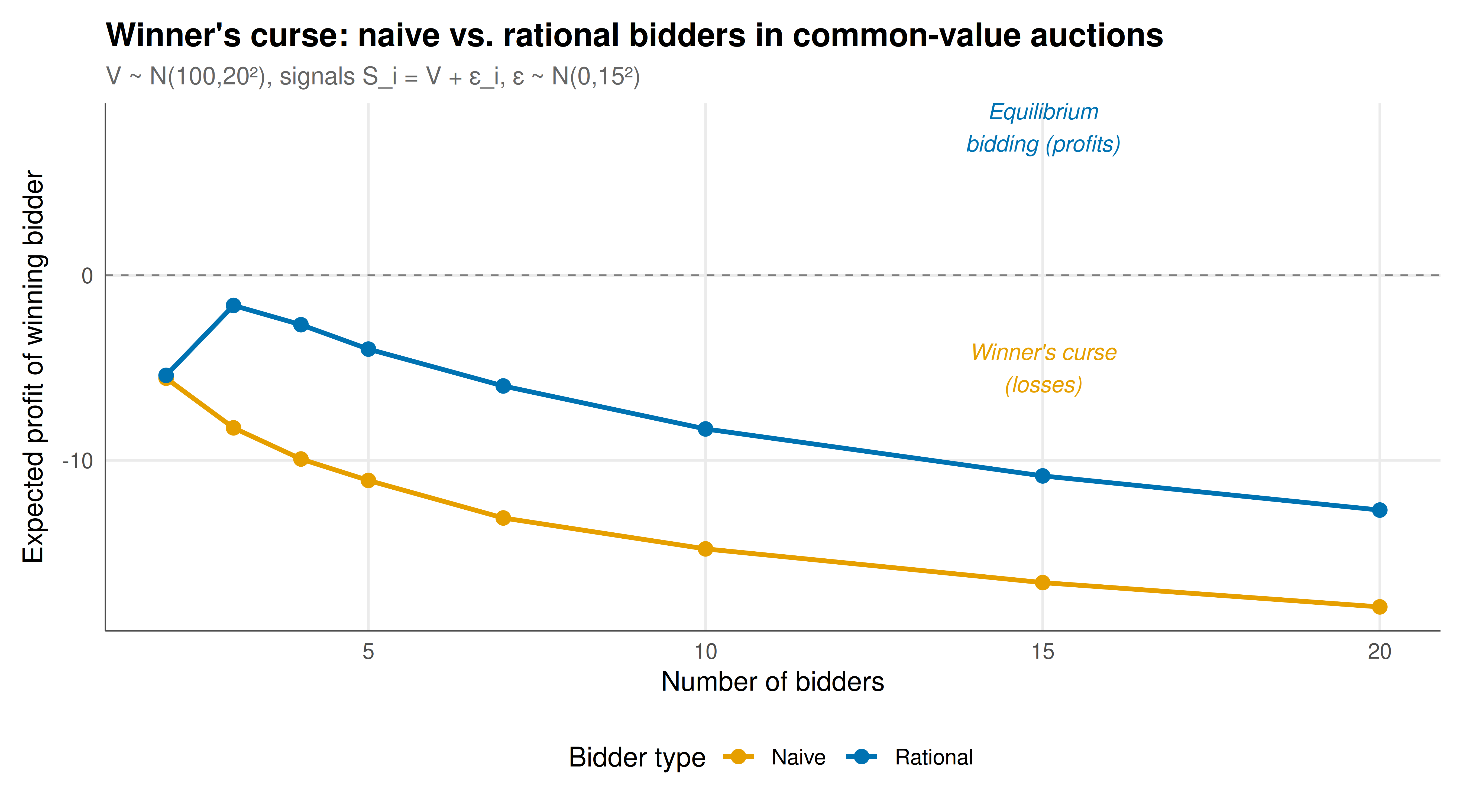
We visualize the expected profit of naive versus rational bidders as a function of the number of bidders, clearly showing the winner's curse.
```{r}
#| label: fig-winners-curse
#| fig-cap: "Figure 1. The winner's curse in common-value first-price auctions. Orange: expected profit of naive bidders who ignore the informational content of winning. Blue: expected profit of rational bidders who condition on winning. As the number of bidders increases, the winner's signal becomes a more extreme order statistic, amplifying the upward bias. Naive bidders suffer increasing losses while rational bidders maintain positive (though declining) expected profits. Dashed line at zero separates profit from loss."
#| dev: [png, pdf]
#| fig-width: 9
#| fig-height: 5
#| dpi: 300
curse_long <- curse_df |>
  select(n_bidders, Naive = naive_profit, Rational = rational_profit) |>
  pivot_longer(-n_bidders, names_to = "Bidder_type", values_to = "Expected_profit")

p_curse <- ggplot(curse_long, aes(x = n_bidders, y = Expected_profit,
                                   color = Bidder_type)) +
  geom_line(linewidth = 1) +
  geom_point(size = 2.5) +
  geom_hline(yintercept = 0, linetype = "dashed", color = "grey50", linewidth = 0.4) +
  scale_color_manual(values = c("Naive" = okabe_ito[1], "Rational" = okabe_ito[5]),
                     name = "Bidder type") +
  annotate("text", x = 15, y = -5,
           label = "Winner's curse\n(losses)", color = okabe_ito[1],
           size = 3.5, fontface = "italic") +
  annotate("text", x = 15, y = 8,
           label = "Equilibrium\nbidding (profits)", color = okabe_ito[5],
           size = 3.5, fontface = "italic") +
  labs(
    title = "Winner's curse: naive vs. rational bidders in common-value auctions",
    subtitle = paste0("V ~ N(", mu_V, ",", sigma_V, "\u00b2), signals S_i = V + \u03b5_i, ",
                      "\u03b5 ~ N(0,", sigma_eps, "\u00b2)"),
    x = "Number of bidders",
    y = "Expected profit of winning bidder"
  ) +
  theme_publication()

p_curse
```
## Interactive figure
The interactive figure shows the joint distribution of the winner's signal, true value, and profit for a specific auction setting, allowing exploration of individual auction outcomes.
```{r}
#| label: fig-curse-interactive
# Combine naive and rational results for n=5
combined_5 <- bind_rows(naive_5, rational_5)

# Sample for plotting (too many points for plotly)
set.seed(42)
sample_idx <- sample(nrow(naive_5), 3000)

plot_data <- bind_rows(
  naive_5[sample_idx, ] |> mutate(type = "Naive"),
  rational_5[sample_idx, ] |> mutate(type = "Rational")
)

plot_data <- plot_data |>
  mutate(text = sprintf("True value: %.1f\nWinning signal: %.1f\nBid: %.1f\nProfit: %.1f\nType: %s",
                         V, winning_signal, winning_bid, profit, type))

p_scatter <- ggplot(plot_data, aes(x = winning_signal, y = profit,
                                    color = type, text = text)) +
  geom_point(alpha = 0.15, size = 0.8) +
  geom_hline(yintercept = 0, linetype = "dashed", color = "grey50") +
  geom_smooth(method = "loess", se = FALSE, linewidth = 1, span = 0.3) +
  scale_color_manual(values = c("Naive" = okabe_ito[1], "Rational" = okabe_ito[5]),
                     name = "Bidder type") +
  labs(
    title = "Profit vs. winning signal in common-value auctions (n=5)",
    subtitle = "Each dot is one auction; curves show conditional mean profit",
    x = "Winner's signal",
    y = "Profit (V - bid)"
  ) +
  theme_publication()

ggplotly(p_scatter, tooltip = "text") |>
  config(displaylogo = FALSE,
         modeBarButtonsToRemove = c("select2d", "lasso2d"))
```
## Interpretation
The simulation results paint a stark picture of the winner's curse in action. With $n = 5$ bidders, naive bidders who bid their Bayesian posterior mean $E[V | S_i]$ without conditioning on the event of winning suffer average losses of several monetary units per auction. The root cause is clearly visible in the signal bias statistic: the winning signal exceeds the true value by a substantial amount on average, because the winning signal is the maximum of $n$ noisy estimates. This upward bias is not a flaw in the individual estimates — each bidder's signal is an unbiased estimate of $V$ — but rather a selection effect: by conditioning on having the highest signal, the winner selects for positive noise realizations.
The scaling with the number of bidders is particularly instructive. As $n$ grows, the expected value of the maximum of $n$ standard normal variables grows approximately as $\sqrt{2 \ln n}$, which means the winner's signal bias grows without bound (albeit slowly). For naive bidders, this translates into steadily increasing losses. With 20 bidders, the average naive bidder profit is deeply negative — a strong incentive to either shade bids or avoid participating altogether. Rational bidders, by contrast, account for this bias by reducing their bids. Their expected profit remains positive but declines with $n$ because competition becomes more intense and the informational advantage of having the highest signal shrinks.
The interactive scatter plot reveals another important feature: the winner's curse is not a constant — it varies with the level of the winning signal. When the winning signal is very high, the true value is likely high as well (but not as high as the signal suggests), and the curse is roughly proportional to the signal level. When the winning signal is near the prior mean $\mu_V$, the curse is smaller because there is less scope for the signal to overestimate $V$. This heterogeneity in curse magnitude across signal levels is captured by the rational bidding strategy, which applies a signal-dependent correction. The practical takeaway for real-world bidders — in oil lease auctions, corporate acquisitions, and procurement — is that failing to condition on the event of winning is not merely a theoretical curiosity but a reliable path to financial ruin.
## Extensions & related tutorials
- [Revenue equivalence theorem](../revenue-equivalence/) — the benchmark result for private-value auctions that breaks down in the common-value setting.
- [First-price sealed-bid auctions](../first-price-sealed-bid/) — the auction format used in this tutorial, with detailed analysis of private-value equilibria.
- [GSP auction for online advertising](../gsp-auction/) — a multi-unit format where common-value elements arise through click-through rate estimation.
- [Signaling games and perfect Bayesian equilibrium](../../foundations/signaling-games-pbe/) — the broader information economics framework of which the winner's curse is a special case.
- [Nash equilibrium in mixed strategies](../../foundations/nash-equilibrium-mixed/) — the equilibrium concept underlying bidding strategies in common-value auctions.
## References
::: {#refs}
:::