---
title: "Signaling games and perfect Bayesian equilibrium"
description: "Model strategic communication under asymmetric information in R, compute perfect Bayesian equilibria with separating and pooling strategies, and visualize how informed players signal their types."
author: "Raban Heller"
date: 2026-05-08
date-modified: 2026-05-08
categories:
- foundations
- signaling-games
- perfect-bayesian-equilibrium
- incomplete-information
keywords: ["signaling game", "perfect Bayesian equilibrium", "PBE", "separating equilibrium", "pooling equilibrium", "Spence"]
labels: ["equilibrium-concepts", "incomplete-information"]
tier: 1
bibliography: ../../../references.bib
vgwort: "TODO_VGWORT_foundations_signaling-games-pbe"
image: thumbnail.png
image-alt: "Signaling game tree with separating and pooling equilibrium paths highlighted"
citation:
type: webpage
url: https://r-heller.github.io/equilibria/tutorials/foundations/signaling-games-pbe/
license: "CC BY-SA 4.0"
draft: false
has_static_fig: true
has_interactive_fig: true
has_shiny_app: false
---
```{r}
#| label: setup
#| include: false
library(ggplot2)
library(dplyr)
library(tidyr)
library(plotly)
okabe_ito <- c("#E69F00", "#56B4E9", "#009E73", "#F0E442",
"#0072B2", "#D55E00", "#CC79A7", "#999999")
theme_publication <- function(base_size = 12) {
theme_minimal(base_size = base_size) +
theme(plot.title = element_text(size = base_size * 1.2, face = "bold"),
plot.subtitle = element_text(size = base_size * 0.9, color = "grey40"),
axis.line = element_line(color = "grey30", linewidth = 0.3),
panel.grid.minor = element_blank(), legend.position = "bottom",
plot.margin = margin(10, 10, 10, 10))
}
```
## Introduction & motivation
In many strategic situations, one party knows something the other does not — and can take costly actions to credibly reveal (or conceal) that information. Michael Spence's 1973 job-market signaling model showed that high-ability workers may invest in education not because it raises productivity, but because it credibly signals their type to employers who cannot directly observe ability. This insight — that costly actions can serve as credible communication devices — pervades economics: firms signal quality through warranties, governments signal resolve through military mobilisation, and startups signal viability through burning cash. The formal analysis of such situations uses **signaling games**, a class of dynamic games of incomplete information where an informed Sender moves first (choosing a signal), and an uninformed Receiver updates beliefs and responds. The equilibrium concept is **perfect Bayesian equilibrium** (PBE): strategies must be sequentially rational given beliefs, and beliefs must be consistent with strategies via Bayes' rule wherever possible. PBE refines the Bayes-Nash equilibrium concept for sequential games by requiring that players' beliefs at every information set are explicitly specified and updated. The key distinction is between **separating equilibria** (different types send different signals, fully revealing their private information) and **pooling equilibria** (all types send the same signal, leaving the Receiver unable to distinguish them). This tutorial implements Spence's signaling model in R, computes both equilibrium types, analyses the conditions under which each survives equilibrium refinements, and visualizes how the signaling cost structure determines which equilibrium prevails.
## Mathematical formulation
A **signaling game** has: a Sender with type $\theta \in \{\theta_L, \theta_H\}$ drawn from prior $p(\theta_H) = \pi$; a signal space $M$; and a Receiver who observes the signal $m$ and chooses action $a \in A$.
A **perfect Bayesian equilibrium** is: (i) a Sender strategy $\sigma^*: \Theta \to \Delta(M)$; (ii) a Receiver strategy $\alpha^*: M \to \Delta(A)$; (iii) a belief system $\mu: M \to \Delta(\Theta)$ such that:
1. **Sequential rationality (Sender)**: $\sigma^*(\theta) \in \arg\max_m u_S(\theta, m, \alpha^*(m))$
2. **Sequential rationality (Receiver)**: $\alpha^*(m) \in \arg\max_a \sum_\theta \mu(\theta|m) u_R(\theta, m, a)$
3. **Belief consistency**: $\mu(\theta|m) = \frac{p(\theta)\sigma^*(m|\theta)}{\sum_{\theta'} p(\theta')\sigma^*(m|\theta')}$ for signals on the equilibrium path.
**Spence's education model**: Worker type $\theta \in \{\theta_L, \theta_H\}$ with productivity $\theta_H > \theta_L > 0$. Education signal $e \geq 0$ costs $c(e, \theta) = e/\theta$ (cheaper for high types). Employer pays wage $w = E[\theta|e]$.
- **Separating PBE**: $e^*(\theta_L) = 0$, $e^*(\theta_H) = e^* \in [\theta_L(\theta_H - \theta_L), \theta_H(\theta_H - \theta_L)]$. Employer pays $w(0) = \theta_L$, $w(e^*) = \theta_H$.
- **Pooling PBE**: Both types choose $e = 0$. Employer pays $w = \pi\theta_H + (1-\pi)\theta_L$.
## R implementation
```{r}
#| label: signaling-game
# --- Spence signaling model ---
theta_L <- 1   # low-type productivity
theta_H <- 2   # high-type productivity
pi_H <- 0.5    # prior on high type

# Signaling cost: c(e, theta) = e / theta
signal_cost <- function(e, theta) e / theta

# --- Separating equilibrium ---
# High type must signal enough that low type won't mimic
# IC for low type: theta_L - 0 >= theta_H - e*/theta_L  =>  e* >= theta_L*(theta_H - theta_L)
# IC for high type: theta_H - e*/theta_H >= theta_L - 0  =>  e* <= theta_H*(theta_H - theta_L)

e_min_sep <- theta_L * (theta_H - theta_L)
e_max_sep <- theta_H * (theta_H - theta_L)

cat("=== Spence Signaling Model ===\n")
cat(sprintf("Types: θ_L = %.0f, θ_H = %.0f, P(θ_H) = %.1f\n", theta_L, theta_H, pi_H))
cat(sprintf("\n--- Separating Equilibrium ---\n"))
cat(sprintf("Education range for high type: e* ∈ [%.1f, %.1f]\n", e_min_sep, e_max_sep))
cat(sprintf("Least-cost separating: e* = %.1f\n", e_min_sep))
# Payoffs under separating (least-cost)
e_star <- e_min_sep
payoff_L_sep <- theta_L - signal_cost(0, theta_L)     # low type: wage θ_L, no education
payoff_H_sep <- theta_H - signal_cost(e_star, theta_H)  # high type: wage θ_H, education e*

cat(sprintf("Low type: wage = %.1f, cost = 0, payoff = %.2f\n", theta_L, payoff_L_sep))
cat(sprintf("High type: wage = %.1f, cost = %.2f, payoff = %.2f\n",
            theta_H, signal_cost(e_star, theta_H), payoff_H_sep))
# --- Pooling equilibrium ---
w_pool <- pi_H * theta_H + (1 - pi_H) * theta_L

cat(sprintf("\n--- Pooling Equilibrium (e = 0) ---\n"))
cat(sprintf("Pooling wage: w = %.2f\n", w_pool))
payoff_L_pool <- w_pool
payoff_H_pool <- w_pool
cat(sprintf("Low type payoff: %.2f (gains %.2f vs separating)\n",
            payoff_L_pool, payoff_L_pool - payoff_L_sep))
cat(sprintf("High type payoff: %.2f (loses %.2f vs separating)\n",
            payoff_H_pool, payoff_H_sep - payoff_H_pool))
# --- Welfare comparison ---
welfare_sep <- 0.5 * payoff_L_sep + 0.5 * payoff_H_sep
welfare_pool <- 0.5 * payoff_L_pool + 0.5 * payoff_H_pool
cat(sprintf("\nExpected welfare: separating = %.3f, pooling = %.3f\n", welfare_sep, welfare_pool))
cat("(Separating equilibrium is inefficient: education is pure signaling waste)\n")
```
## Static publication-ready figure
```{r}
#| label: fig-signaling-equilibria
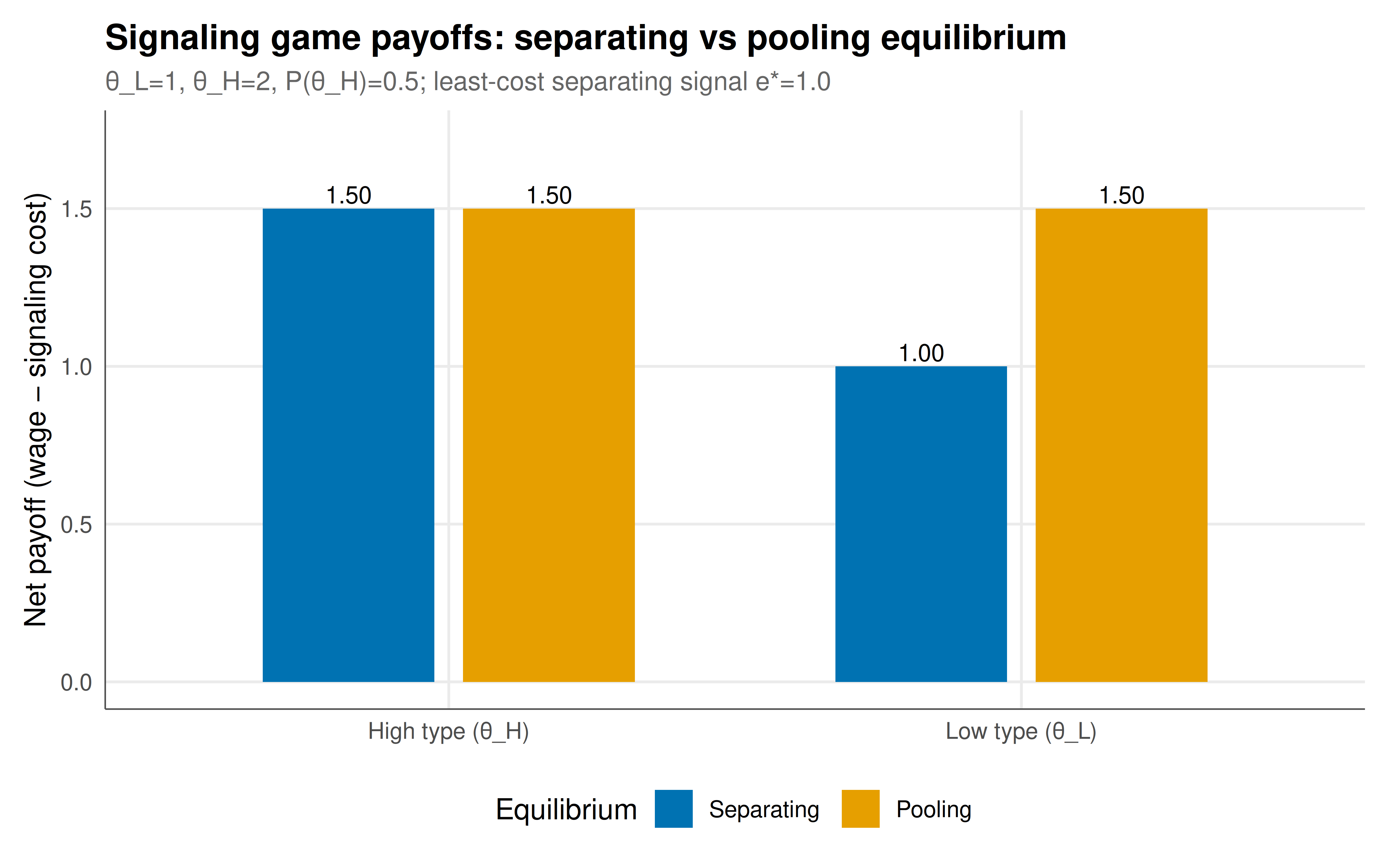
#| fig-cap: "Figure 1. Spence's education signaling model: separating vs pooling equilibrium payoffs for each worker type. In the separating equilibrium, the high-type worker invests in education to credibly signal ability, earning a higher wage but bearing signaling costs. In the pooling equilibrium, both types earn the average wage — benefiting the low type at the high type's expense. The separating equilibrium is socially inefficient because education is pure waste (no productivity effect). Okabe-Ito palette."
#| dev: [png, pdf]
#| fig-width: 8
#| fig-height: 5
#| dpi: 300
# Build comparison data
eq_data <- tibble(
  type = rep(c("Low type (θ_L)", "High type (θ_H)"), 2),
  equilibrium = rep(c("Separating", "Pooling"), each = 2),
  wage = c(theta_L, theta_H, w_pool, w_pool),
  cost = c(0, signal_cost(e_star, theta_H), 0, 0),
  payoff = c(payoff_L_sep, payoff_H_sep, payoff_L_pool, payoff_H_pool)
) |> mutate(
  equilibrium = factor(equilibrium, levels = c("Separating", "Pooling")),
  component = "Payoff"
)

# Stacked: wage minus cost = payoff
bar_data <- eq_data |>
  select(type, equilibrium, payoff) |>
  mutate(label = sprintf("%.2f", payoff))

ggplot(bar_data, aes(x = type, y = payoff, fill = equilibrium)) +
  geom_col(position = position_dodge(width = 0.7), width = 0.6) +
  geom_text(aes(label = label), position = position_dodge(width = 0.7),
            vjust = -0.3, size = 3.5) +
  scale_fill_manual(values = c("Separating" = okabe_ito[5], "Pooling" = okabe_ito[1]),
                     name = "Equilibrium") +
  labs(title = "Signaling game payoffs: separating vs pooling equilibrium",
       subtitle = sprintf("θ_L=%d, θ_H=%d, P(θ_H)=%.1f; least-cost separating signal e*=%.1f",
                           theta_L, theta_H, pi_H, e_star),
       x = NULL, y = "Net payoff (wage − signaling cost)") +
  coord_cartesian(ylim = c(0, max(bar_data$payoff) * 1.15)) +
  theme_publication()
```
## Interactive figure
```{r}
#| label: fig-signaling-sensitivity
# How does the separating equilibrium range change with type spread?
theta_H_seq <- seq(1.1, 4, by = 0.05)
sep_data <- lapply(theta_H_seq, function(tH) {
  e_min <- theta_L * (tH - theta_L)
  e_max <- tH * (tH - theta_L)
  e_lc <- e_min  # least-cost separating
  payoff_H <- tH - e_lc / tH
  payoff_pool <- 0.5 * tH + 0.5 * theta_L
  tibble(theta_H = tH, e_min = e_min, e_max = e_max,
         payoff_sep_H = payoff_H, payoff_pool_H = payoff_pool)
}) |> bind_rows() |>
  pivot_longer(c(payoff_sep_H, payoff_pool_H),
               names_to = "equilibrium", values_to = "payoff") |>
  mutate(
    eq_label = ifelse(equilibrium == "payoff_sep_H", "Separating", "Pooling"),
    text = paste0("θ_H = ", round(theta_H, 2),
                  "\nEquilibrium: ", eq_label,
                  "\nHigh-type payoff: ", round(payoff, 3))
  )

p_sens <- ggplot(sep_data, aes(x = theta_H, y = payoff, color = eq_label, text = text)) +
  geom_line(linewidth = 1) +
  scale_color_manual(values = c("Separating" = okabe_ito[5], "Pooling" = okabe_ito[1]),
                      name = "Equilibrium") +
  labs(title = "High-type payoff: separating vs pooling as type spread varies",
       subtitle = "As θ_H increases, separating becomes more attractive (signaling cost grows slower than wage gain)",
       x = "High-type productivity (θ_H)", y = "High-type net payoff") +
  theme_publication()

ggplotly(p_sens, tooltip = "text") |>
  config(displaylogo = FALSE, modeBarButtonsToRemove = c("select2d", "lasso2d"))
```
## Interpretation
Signaling games formalize one of the deepest insights in information economics: when direct communication is cheap (costless talk), it is often not credible, but costly actions can serve as credible signals precisely because they are differentially costly across types. In Spence's model, education works as a signal not because it makes workers more productive, but because high-ability workers find it less costly to acquire — creating a natural screening device. The separating equilibrium is informationally efficient (employers learn the worker's true type) but socially wasteful (education resources are burned purely for signaling). The pooling equilibrium avoids this waste but creates adverse selection: high types subsidise low types through the averaged wage, potentially driving high types out of the market. The tension between these equilibria is resolved by **equilibrium refinements** — the Cho-Kreps intuitive criterion eliminates many pooling equilibria by requiring "reasonable" off-path beliefs, typically selecting the least-cost separating equilibrium as the unique surviving outcome. The sensitivity analysis reveals that signaling becomes more attractive to the high type as the productivity gap widens: the wage premium from separation grows linearly in $\theta_H$, while the signaling cost grows sub-linearly (because $e^*/\theta_H = \theta_L(1 - \theta_L/\theta_H)$ is bounded). Perfect Bayesian equilibrium is the workhorse solution concept for these sequential incomplete-information games — it extends subgame perfection by requiring explicit beliefs at every information set and Bayesian updating on the equilibrium path, while leaving off-path beliefs as a degree of freedom that refinements then discipline.
## Extensions & related tutorials
- [Bayesian games and incomplete information](../../bayesian-methods/bayesian-games-incomplete-information/) — the simultaneous-move counterpart.
- [Extensive-form games and subgame perfection](../extensive-form-subgame-perfection/) — the complete-information foundation.
- [Cuban Missile Crisis as signaling game](../../real-world-data-applications/cuban-missile-crisis-signaling-game/) — applied signaling analysis.
- [Mechanism design introduction](../../mechanism-design/mechanism-design-intro/) — designing rules to elicit private information.
- [Vickrey auction and DSIC](../../mechanism-design/vickrey-second-price-auction/) — mechanism design with dominant strategies.
## References
::: {#refs}
:::