---
title: "The Vickrey (second-price) auction — truth-telling as a dominant strategy"
description: "Analyse the Vickrey sealed-bid second-price auction in R, prove that truthful bidding is a weakly dominant strategy, simulate revenue comparisons with first-price auctions, and visualize bidding equilibria."
author: "Raban Heller"
date: 2026-05-08
date-modified: 2026-05-08
categories:
- mechanism-design
- auctions
- vickrey
- dominant-strategy
keywords: ["Vickrey auction", "second-price auction", "truthful bidding", "mechanism design", "revenue equivalence", "DSIC"]
labels: ["mechanism-design", "auction-theory"]
tier: 1
bibliography: ../../../references.bib
vgwort: "TODO_VGWORT_mechanism-design_vickrey-second-price-auction"
image: thumbnail.png
image-alt: "Bid distribution comparison between first-price and second-price sealed-bid auctions"
citation:
type: webpage
url: https://r-heller.github.io/equilibria/tutorials/mechanism-design/vickrey-second-price-auction/
license: "CC BY-SA 4.0"
draft: false
has_static_fig: true
has_interactive_fig: true
has_shiny_app: false
---
```{r}
#| label: setup
#| include: false
library(ggplot2)
library(dplyr)
library(tidyr)
library(plotly)
okabe_ito <- c("#E69F00", "#56B4E9", "#009E73", "#F0E442",
"#0072B2", "#D55E00", "#CC79A7", "#999999")
theme_publication <- function(base_size = 12) {
theme_minimal(base_size = base_size) +
theme(
plot.title = element_text(size = base_size * 1.2, face = "bold"),
plot.subtitle = element_text(size = base_size * 0.9, color = "grey40"),
axis.line = element_line(color = "grey30", linewidth = 0.3),
panel.grid.minor = element_blank(),
legend.position = "bottom",
plot.margin = margin(10, 10, 10, 10)
)
}
```
## Introduction & motivation
William Vickrey's 1961 analysis of sealed-bid auctions is one of the foundational results in mechanism design — the branch of game theory concerned with designing rules (mechanisms) that elicit desired behaviour from strategic agents. In a **second-price sealed-bid auction** (now called the Vickrey auction), the highest bidder wins but pays the second-highest bid. Vickrey proved a remarkable result: **truthful bidding is a weakly dominant strategy**. Each bidder should bid exactly their private valuation, regardless of what other bidders do, because the payment is determined by someone else's bid. This property — dominant-strategy incentive compatibility (DSIC) — makes the Vickrey auction a gold standard in mechanism design: the auctioneer gets truthful information without requiring bidders to engage in complex strategic reasoning. The Vickrey auction is the intellectual ancestor of Google's ad auctions, eBay's proxy bidding system, and spectrum allocation mechanisms used by governments worldwide. This tutorial proves the dominance of truthful bidding, implements first-price and second-price auction simulations in R, verifies the revenue equivalence theorem via Monte Carlo, and visualizes bidding behaviour across auction formats.
## Mathematical formulation
**Setup**: $n$ bidders with private values $v_1, \ldots, v_n$ drawn independently from distribution $F$ on $[0, \bar{v}]$. Each submits a sealed bid $b_i$.
**Second-price auction**: Winner $= \arg\max_i b_i$; payment $= \max_{j \neq i} b_j$ (second-highest bid).
**Proposition**: Bidding $b_i = v_i$ is a weakly dominant strategy.
*Proof*: Consider bidder $i$ with value $v_i$. Let $m = \max_{j \neq i} b_j$ be the highest competing bid. Three cases:
1. $v_i > m$: Bidding $v_i$ wins, pays $m$, surplus = $v_i - m > 0$. Any bid $b_i > m$ also wins with same payment. Bidding $b_i < m$ loses, surplus = 0. Truth-telling is weakly best.
2. $v_i < m$: Bidding $v_i$ loses, surplus = 0. Any bid $b_i > m$ wins but pays $m > v_i$, surplus < 0. Truth-telling avoids this loss.
3. $v_i = m$: Indifferent between winning (surplus 0) and losing (surplus 0). $\square$
**First-price auction**: Winner pays their own bid. Equilibrium bid with $n$ bidders and $v_i \sim U[0,1]$: $b_i^*(v_i) = \frac{n-1}{n} v_i$ (shade by $1/n$).
**Revenue Equivalence Theorem**: Under independent private values, any auction that allocates to the highest-value bidder and gives zero surplus to the lowest type yields the same expected revenue: $E[R] = E[\text{2nd highest value}]$.
## R implementation
```{r}
#| label: auction-simulations
set.seed(42)
n_bidders <- 5
n_simulations <- 10000

# Simulate auctions with values from U[0,1]
simulate_auctions <- function(n_bidders, n_sims) {
  results <- lapply(1:n_sims, function(s) {
    values <- sort(runif(n_bidders), decreasing = TRUE)

    # Second-price: truthful bidding
    sp_winner_value <- values[1]
    sp_payment <- values[2]
    sp_surplus <- sp_winner_value - sp_payment

    # First-price: equilibrium bidding b = (n-1)/n * v
    bids_fp <- ((n_bidders - 1) / n_bidders) * values
    fp_winner_idx <- which.max(bids_fp)
    fp_payment <- bids_fp[fp_winner_idx]
    fp_surplus <- values[fp_winner_idx] - fp_payment

    tibble(
      sim = s,
      sp_revenue = sp_payment,
      fp_revenue = fp_payment,
      sp_surplus = sp_surplus,
      fp_surplus = fp_surplus,
      winner_value = sp_winner_value,
      second_value = values[2]
    )
  }) |> bind_rows()

  results
}

results <- simulate_auctions(n_bidders, n_simulations)

cat(sprintf("=== Auction Simulation: %d bidders, %d auctions, values ~ U[0,1] ===\n\n",
            n_bidders, n_simulations))
cat(sprintf("Second-price auction:\n  Mean revenue: %.4f\n  Mean winner surplus: %.4f\n",
            mean(results$sp_revenue), mean(results$sp_surplus)))
cat(sprintf("\nFirst-price auction (equilibrium bidding):\n  Mean revenue: %.4f\n  Mean winner surplus: %.4f\n",
            mean(results$fp_revenue), mean(results$fp_surplus)))
cat(sprintf("\nTheoretical expected revenue (both): %.4f\n",
            (n_bidders - 1) / (n_bidders + 1)))
cat("(Revenue equivalence confirmed!)\n")
```
## Static publication-ready figure
```{r}
#| label: fig-auction-comparison
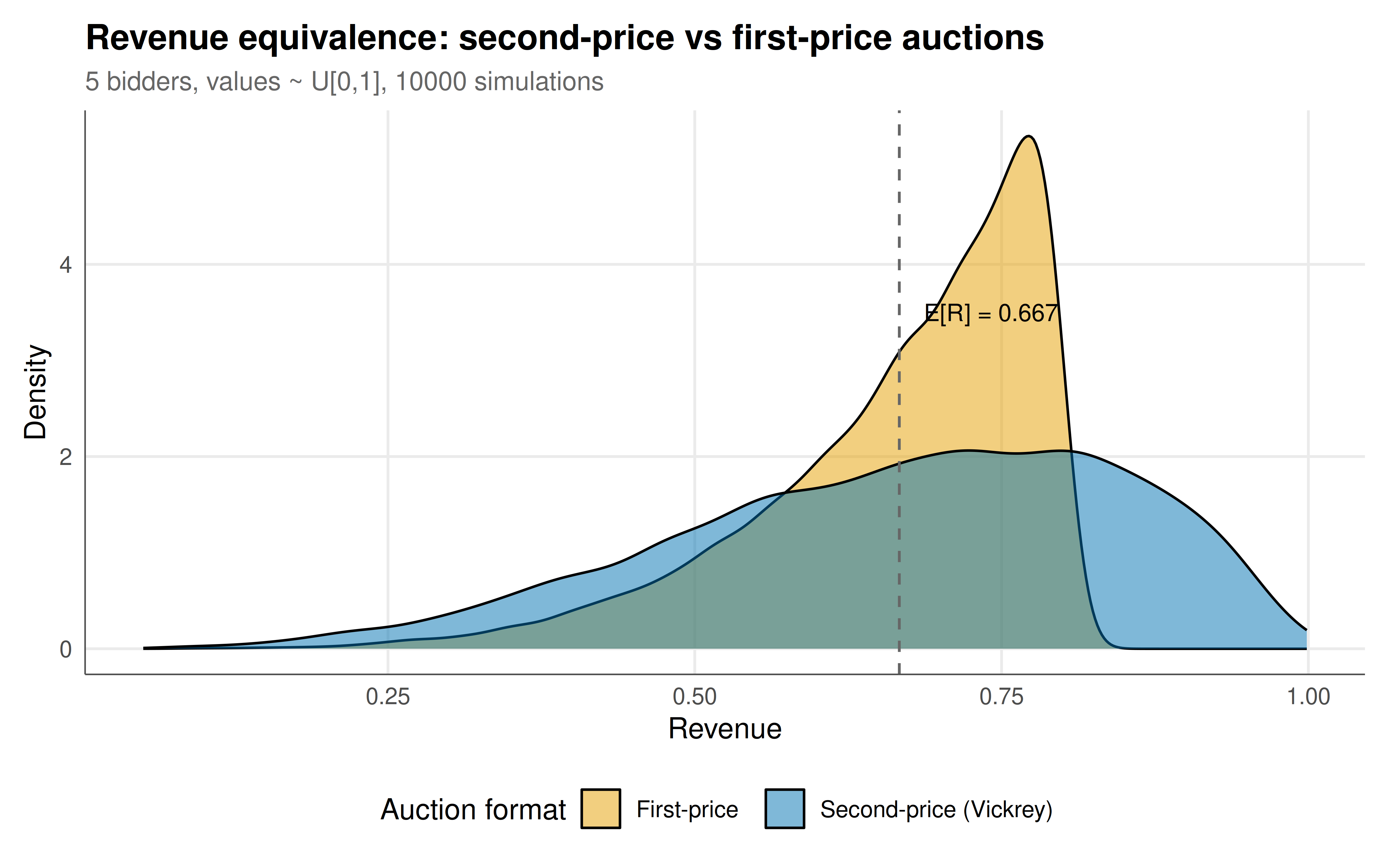
#| fig-cap: "Figure 1. Revenue distributions for second-price (Vickrey) and first-price auctions with 5 bidders and values drawn uniformly from [0, 1]. The revenue equivalence theorem predicts identical expected revenue (dashed line), confirmed by the simulation. The second-price auction has higher variance because payment depends on a single order statistic. Okabe-Ito palette."
#| dev: [png, pdf]
#| fig-width: 8
#| fig-height: 5
#| dpi: 300
revenue_long <- results |>
  select(sim, sp_revenue, fp_revenue) |>
  pivot_longer(-sim, names_to = "auction", values_to = "revenue") |>
  mutate(auction = ifelse(auction == "sp_revenue", "Second-price (Vickrey)", "First-price"))

theoretical_rev <- (n_bidders - 1) / (n_bidders + 1)

p_rev <- ggplot(revenue_long, aes(x = revenue, fill = auction)) +
  geom_density(alpha = 0.5, linewidth = 0.5) +
  geom_vline(xintercept = theoretical_rev, linetype = "dashed", color = "grey40") +
  annotate("text", x = theoretical_rev + 0.02, y = 3.5,
           label = sprintf("E[R] = %.3f", theoretical_rev),
           size = 3.5, hjust = 0) +
  scale_fill_manual(values = c("Second-price (Vickrey)" = okabe_ito[5],
                                "First-price" = okabe_ito[1]),
                     name = "Auction format") +
  labs(
    title = "Revenue equivalence: second-price vs first-price auctions",
    subtitle = sprintf("%d bidders, values ~ U[0,1], %d simulations", n_bidders, n_simulations),
    x = "Revenue", y = "Density"
  ) +
  theme_publication()

p_rev
```
## Interactive figure
```{r}
#| label: fig-bidding-strategies
# Visualize equilibrium bidding strategies across auction formats
v_seq <- seq(0, 1, by = 0.01)

bid_strategies <- tibble(
  value = rep(v_seq, 3),
  auction = rep(c("Second-price (bid = v)",
                   "First-price (n=3): bid = 2v/3",
                   "First-price (n=10): bid = 9v/10"), each = length(v_seq)),
  bid = c(v_seq, 2/3 * v_seq, 9/10 * v_seq)
) |>
  mutate(text = paste0("Value: ", round(value, 2),
                       "\nBid: ", round(bid, 2),
                       "\nFormat: ", auction))

p_bids <- ggplot(bid_strategies, aes(x = value, y = bid, color = auction, text = text)) +
  geom_line(linewidth = 1) +
  geom_abline(slope = 1, intercept = 0, linetype = "dotted", color = "grey60") +
  scale_color_manual(values = okabe_ito[c(5, 1, 6)], name = "Auction format") +
  labs(
    title = "Equilibrium bidding strategies by auction format",
    subtitle = "Second-price: bid truthfully (45° line). First-price: shade below value; more bidders → less shading.",
    x = "Private value (v)", y = "Equilibrium bid (b)"
  ) +
  theme_publication()

ggplotly(p_bids, tooltip = "text") |>
  config(displaylogo = FALSE,
         modeBarButtonsToRemove = c("select2d", "lasso2d"))
```
## Interpretation
The Vickrey auction's elegance lies in its simplicity: by decoupling the payment from the winner's own bid, it removes all incentives for strategic manipulation. A bidder who overbids risks winning at a price above their value (negative surplus); a bidder who underbids risks losing when they should have won. Truth-telling is the unique strategy that avoids both dangers, making it weakly dominant — no information about other bidders' strategies or values is needed. The simulation confirms the revenue equivalence theorem: despite the dramatically different bidding strategies (truthful in second-price, shaded by $1/n$ in first-price), expected revenue is identical. However, the revenue distributions differ — the second-price auction has higher variance because payment is a single order statistic, while the first-price auction's payment is a continuous function of the winner's value, smoothing out extremes. The bidding strategy plot reveals the economic intuition behind first-price bid shading: with more competitors ($n = 10$), bidders shade less ($b = 0.9v$) because competition forces bids closer to values. In the limit of infinite bidders, both auctions converge to payment equal to the winner's value (zero surplus). The Vickrey mechanism's DSIC property makes it the conceptual starting point for all of mechanism design — from the VCG (Vickrey-Clarke-Groves) mechanism for multi-item allocation to Google's generalised second-price auction for online advertising, to spectrum auctions where governments sell billions of dollars in radio frequencies.
## Extensions & related tutorials
- [Dominant strategies and IESDS](../../foundations/dominant-strategies-iterated-elimination/) — the dominance concept underlying DSIC.
- [First-price auction equilibrium](../../auction-theory-deep-dive/first-price-sealed-bid/) — deriving the bid-shading formula.
- [VCG mechanism](../vcg-mechanism/) — generalising Vickrey to multi-item settings.
- [Revenue equivalence theorem](../../auction-theory-deep-dive/revenue-equivalence/) — formal proof and extensions.
- [Google ad auctions](../../auction-theory-deep-dive/gsp-auction/) — the practical descendant of Vickrey.
## References
::: {#refs}
:::