---
title: "Hyperbolic discounting and time-inconsistent strategic behaviour"
description: "Model quasi-hyperbolic (beta,delta) preferences in strategic settings, find Markov perfect equilibria of intrapersonal games, and compare exponential vs hyperbolic discounters in repeated interactions."
author: "Raban Heller"
date: 2026-05-08
date-modified: 2026-05-08
categories:
- behavioral-economics
- hyperbolic-discounting
- time-inconsistency
- commitment
keywords: ["hyperbolic discounting", "quasi-hyperbolic preferences", "present bias", "time inconsistency", "Markov perfect equilibrium"]
labels: ["behavioral-game-theory", "intertemporal-choice"]
tier: 1
bibliography: ../../../references.bib
vgwort: "TODO_VGWORT_behavioral-economics_hyperbolic-discounting-games"
image: thumbnail.png
image-alt: "Comparison of exponential and hyperbolic discount functions showing the present bias gap"
citation:
type: webpage
url: https://r-heller.github.io/equilibria/tutorials/behavioral-economics/hyperbolic-discounting-games/
license: "CC BY-SA 4.0"
draft: false
has_static_fig: true
has_interactive_fig: true
has_shiny_app: false
---
```{r}
#| label: setup
#| include: false
library(ggplot2)
library(dplyr)
library(tidyr)
library(plotly)
okabe_ito <- c("#E69F00", "#56B4E9", "#009E73", "#F0E442",
"#0072B2", "#D55E00", "#CC79A7", "#999999")
theme_publication <- function(base_size = 12) {
theme_minimal(base_size = base_size) +
theme(plot.title = element_text(size = base_size * 1.2, face = "bold"),
plot.subtitle = element_text(size = base_size * 0.9, color = "grey40"),
axis.line = element_line(color = "grey30", linewidth = 0.3),
panel.grid.minor = element_blank(), legend.position = "bottom",
plot.margin = margin(10, 10, 10, 10))
}
```
## Introduction & motivation
Standard economic models assume that agents discount the future exponentially: a reward received $t$ periods from now is worth $\delta^t$ times its face value, where $\delta \in (0,1)$ is the per-period discount factor. Exponential discounting has a critical property called dynamic consistency — a plan that is optimal from today's perspective remains optimal from tomorrow's perspective. If you decide today to start saving next month, you will still want to follow through when next month arrives. This property makes exponential discounting mathematically convenient and normatively appealing, but it fails to describe a robust and pervasive pattern in human behaviour: present bias. People systematically overweight immediate rewards relative to future ones, in a way that exponential discounting cannot capture.
The experimental evidence for present bias is overwhelming and spans decades of research. In classic studies by Thaler (1981) and others, subjects required much larger compensation to delay receiving a reward from today to tomorrow than from day 30 to day 31 — even though both involve a one-day delay. This pattern violates exponential discounting, which predicts that the required compensation depends only on the length of the delay, not on when the delay begins. The preference reversal is characteristic of hyperbolic or quasi-hyperbolic discounting: when a reward is immediate, people place disproportionate weight on it, but when comparing two future dates, they are more patient. Laibson (1997) formalised this pattern with the quasi-hyperbolic or $(\beta, \delta)$ model: the present value of a reward received $t$ periods from now is $\beta \delta^t$ for $t \geq 1$ and $1$ for $t = 0$, where $\beta \in (0,1]$ captures the degree of present bias. When $\beta = 1$, preferences reduce to standard exponential discounting; when $\beta < 1$, there is a "present-bias gap" that creates a wedge between the current self's preferences and those of all future selves.
The strategic implications of present bias are profound and have generated a large literature at the intersection of behavioural economics and game theory. The key insight is that a present-biased agent is effectively playing a game against her own future selves. Today's self wants to save, exercise, and study — starting tomorrow. Tomorrow's self inherits the same bias and again wants to defer. This intrapersonal conflict can be modelled as a sequential game between the current self (player 0) and a sequence of future selves (players 1, 2, ...), each of whom controls the decision in their own period. The appropriate solution concept for this intrapersonal game is the Markov perfect equilibrium (MPE), where each self's strategy depends only on the payoff-relevant state (e.g., current wealth) and is a best response to the strategies of all future selves, who are assumed to be similarly present-biased.
This intrapersonal game perspective, developed by Phelps and Pollak (1968) and Laibson (1997), yields striking results. In a consumption-savings problem, the Markov perfect equilibrium typically involves oversaving relative to the agent's long-run preferences but undersaving relative to the commitment optimum (what the agent would choose if she could bind all future selves). This creates demand for commitment devices — mechanisms that restrict future choices to align with current preferences. Commitment devices include automatic payroll deductions (401(k) plans), illiquid savings accounts, and social contracts (telling friends about your diet). The existence and welfare implications of these devices are central questions in behavioural public economics.
In this tutorial, we implement the $(\beta, \delta)$ model in a savings game where a sequence of selves decides how much to consume and save each period. We find the Markov perfect equilibrium by backward induction over a finite horizon and compare the consumption paths of exponential and hyperbolic discounters. We then explore how present-biased agents perform in a repeated Prisoner's Dilemma, showing that their impatience undermines cooperation even when exponential discounters would sustain it. Finally, we quantify the welfare gains from commitment devices and show that the value of commitment increases with the severity of present bias.
## Mathematical formulation
**Quasi-hyperbolic discounting.** An agent at time $t$ evaluates a stream of utilities $(u_t, u_{t+1}, u_{t+2}, \ldots)$ as:
$$
U_t = u_t + \beta \sum_{\tau=t+1}^{T} \delta^{\tau-t} u_\tau
$$
where $\delta \in (0,1)$ is the long-run discount factor and $\beta \in (0,1]$ is the present-bias parameter. For $\beta = 1$, this reduces to exponential discounting. The discount function is:
$$
D(k) = \begin{cases} 1 & k = 0 \\ \beta \delta^k & k \geq 1 \end{cases}
$$
**Intrapersonal savings game.** Consider a finite-horizon setting with $T$ periods. In each period $t$, the agent has wealth $W_t$ and chooses consumption $c_t \in [0, W_t]$. Savings earn gross return $R > 0$:
$$
W_{t+1} = R \cdot (W_t - c_t)
$$
Utility from consumption is $u(c) = \ln(c)$ (log utility). In the final period $T$, the agent consumes all remaining wealth.
**Markov perfect equilibrium.** In the MPE, each self $t$ takes the strategies of future selves as given and optimises. Let $V_t(W)$ be the value function for self $t$ (the continuation value evaluated using self $t$'s preferences). By backward induction from period $T$:
At $t = T$: $c_T^* = W_T$, $V_T(W) = \ln(W)$.
For $t < T$, self $t$ solves:
$$
\max_{c_t} \; \ln(c_t) + \beta \delta \, V_{t+1}(R(W_t - c_t))
$$
where $V_{t+1}$ is the continuation value under the equilibrium strategies of selves $t+1, \ldots, T$.
**Cooperation in repeated PD.** Two players play a repeated Prisoner's Dilemma with stage payoffs $(R, S, T, P)$ satisfying $T > R > P > S$. With exponential discounting, cooperation is sustainable via grim trigger if $\delta \geq (T - R)/(T - P)$. For $(\beta, \delta)$ discounters, the binding constraint is the current self's temptation:
$$
T - R \leq \beta \delta \frac{R - P}{1 - \delta}
$$
The critical condition becomes $\beta \delta \geq \frac{(T-R)(1-\delta)}{R-P}$, which is harder to satisfy when $\beta < 1$.
## R implementation
```{r}
#| label: savings-game
set.seed(42)

# Parameters
T_horizon <- 20   # Number of periods
R_return <- 1.05   # Gross return on savings
W_init <- 100      # Initial wealth
beta_values <- c(1.0, 0.8, 0.6)  # Present-bias parameters
delta <- 0.95      # Long-run discount factor

# Solve the intrapersonal game by backward induction
solve_savings_mpe <- function(beta, delta, R, T, W_init) {
  # For log utility and linear budget constraint, the MPE consumption rule

  # is c_t = alpha_t * W_t for some alpha_t

  # Backward induction
  alpha <- numeric(T)
  alpha[T] <- 1  # Consume everything in last period

  for (t in (T-1):1) {
    # Self t's optimal consumption share given future selves' strategies
    # FOC: 1/c_t = beta * delta * R / (c_{t+1})
    # In MPE, c_{t+1} = alpha_{t+1} * W_{t+1} = alpha_{t+1} * R * (W_t - c_t)
    # Substituting: 1/(alpha_t * W_t) = beta*delta*R / (alpha_{t+1}*R*(1-alpha_t)*W_t)
    # Simplifying: 1/alpha_t = beta*delta / (alpha_{t+1}*(1-alpha_t))
    # alpha_{t+1}*(1-alpha_t) = beta*delta*alpha_t
    # alpha_{t+1} - alpha_{t+1}*alpha_t = beta*delta*alpha_t
    # alpha_{t+1} = alpha_t*(beta*delta + alpha_{t+1})
    # alpha_t = alpha_{t+1} / (beta*delta + alpha_{t+1})
    alpha[t] <- alpha[t+1] / (beta * delta + alpha[t+1])
  }

  # Simulate forward
  W <- numeric(T)
  C <- numeric(T)
  W[1] <- W_init
  for (t in 1:T) {
    C[t] <- alpha[t] * W[t]
    if (t < T) W[t+1] <- R * (W[t] - C[t])
  }

  data.frame(
    period = 1:T,
    wealth = W,
    consumption = C,
    consumption_share = alpha,
    beta = beta
  )
}

# Solve for each beta
results_list <- lapply(beta_values, function(b) {
  solve_savings_mpe(b, delta, R_return, T_horizon, W_init)
})
results_df <- bind_rows(results_list)
results_df$beta_label <- paste0("beta = ", results_df$beta)

cat("Consumption shares (alpha_t) by period and present-bias:\n")
results_df |>
  filter(period %in% c(1, 5, 10, 15, 20)) |>
  select(period, beta_label, consumption_share) |>
  pivot_wider(names_from = beta_label, values_from = consumption_share) |>
  print()
cat("\nTotal lifetime consumption (present value at t=1):\n")
results_df |>
  group_by(beta_label) |>
  summarise(
    total_consumption = round(sum(consumption), 2),
    first_period_c = round(first(consumption), 2),
    last_period_c = round(last(consumption), 2),
    .groups = "drop"
  ) |>
  print()
```
```{r}
#| label: repeated-pd
# Repeated Prisoner's Dilemma with hyperbolic discounters
# Stage game payoffs
T_pd <- 5   # Temptation
R_pd <- 3   # Reward (mutual cooperation)
P_pd <- 1   # Punishment (mutual defection)
S_pd <- 0   # Sucker's payoff

# Critical discount factor for cooperation (grim trigger)
delta_grid <- seq(0.5, 0.99, by = 0.01)
beta_grid <- c(1.0, 0.9, 0.8, 0.7, 0.6, 0.5)

# For exponential: delta >= (T-R)/(T-P)
delta_crit_exp <- (T_pd - R_pd) / (T_pd - P_pd)

# For (beta,delta): beta*delta*(R-P)/(1-delta) >= T-R
# => beta >= (T-R)*(1-delta) / (delta*(R-P))
coop_data <- expand.grid(delta = delta_grid, beta = beta_grid) |>
  mutate(
    required_patience = (T_pd - R_pd) * (1 - delta) / (delta * (R_pd - P_pd)),
    can_cooperate = beta >= required_patience,
    beta_label = paste0("beta = ", beta)
  )

cat("Critical conditions for cooperation (grim trigger):\n")
cat(sprintf("Exponential: delta >= %.3f\n", delta_crit_exp))
cat("\nMinimum delta for cooperation by beta:\n")
coop_data |>
  group_by(beta_label) |>
  summarise(min_delta = min(delta[can_cooperate], na.rm = TRUE),
            .groups = "drop") |>
  print()
```
```{r}
#| label: commitment-value
# Value of commitment: compare MPE vs commitment (pre-commitment) solution
solve_commitment <- function(delta, R, T, W_init) {
  # Under commitment, the agent maximises sum delta^t ln(c_t)
  # Optimal: c_t = alpha * R^t * (adjusted), standard result
  # For log utility: c_t / c_{t-1} = delta * R (Euler equation)
  alpha_commit <- numeric(T)
  # With commitment and exponential delta: equal effective consumption shares
  # alpha_t = 1 / sum_{s=t}^{T} (delta*R)^{s-t}  (simplified)
  dR <- delta * R
  for (t in 1:T) {
    remaining <- T - t + 1
    if (abs(dR - 1) < 1e-10) {
      alpha_commit[t] <- 1 / remaining
    } else {
      alpha_commit[t] <- (1 - dR) / (1 - dR^remaining)
    }
  }

  W <- numeric(T)
  C <- numeric(T)
  W[1] <- W_init
  for (t in 1:T) {
    C[t] <- alpha_commit[t] * W[t]
    if (t < T) W[t+1] <- R * (W[t] - C[t])
  }

  data.frame(period = 1:T, wealth = W, consumption = C,
             consumption_share = alpha_commit, type = "Commitment")
}

commit_df <- solve_commitment(delta, R_return, T_horizon, W_init)

# Compare welfare (discounted log utility from perspective of self 0)
welfare_comparison <- lapply(beta_values, function(b) {
  mpe <- solve_savings_mpe(b, delta, R_return, T_horizon, W_init)
  # Self 0's evaluation: u_1 + beta * sum_{t=2}^{T} delta^{t-1} u_t
  u_mpe <- log(mpe$consumption)
  welfare_mpe <- u_mpe[1] + b * sum(delta^(1:(T_horizon-1)) * u_mpe[2:T_horizon])

  u_commit <- log(commit_df$consumption)
  welfare_commit <- u_commit[1] + b * sum(delta^(1:(T_horizon-1)) * u_commit[2:T_horizon])

  data.frame(beta = b, welfare_mpe = welfare_mpe,
             welfare_commit = welfare_commit,
             commitment_value = welfare_commit - welfare_mpe)
})

welfare_df <- bind_rows(welfare_comparison)
cat("Welfare comparison (self 0's perspective):\n")
print(welfare_df)
cat("\nThe value of commitment increases as beta decreases (more present bias).\n")
```
## Static publication-ready figure
```{r}
#| label: fig-discount-functions
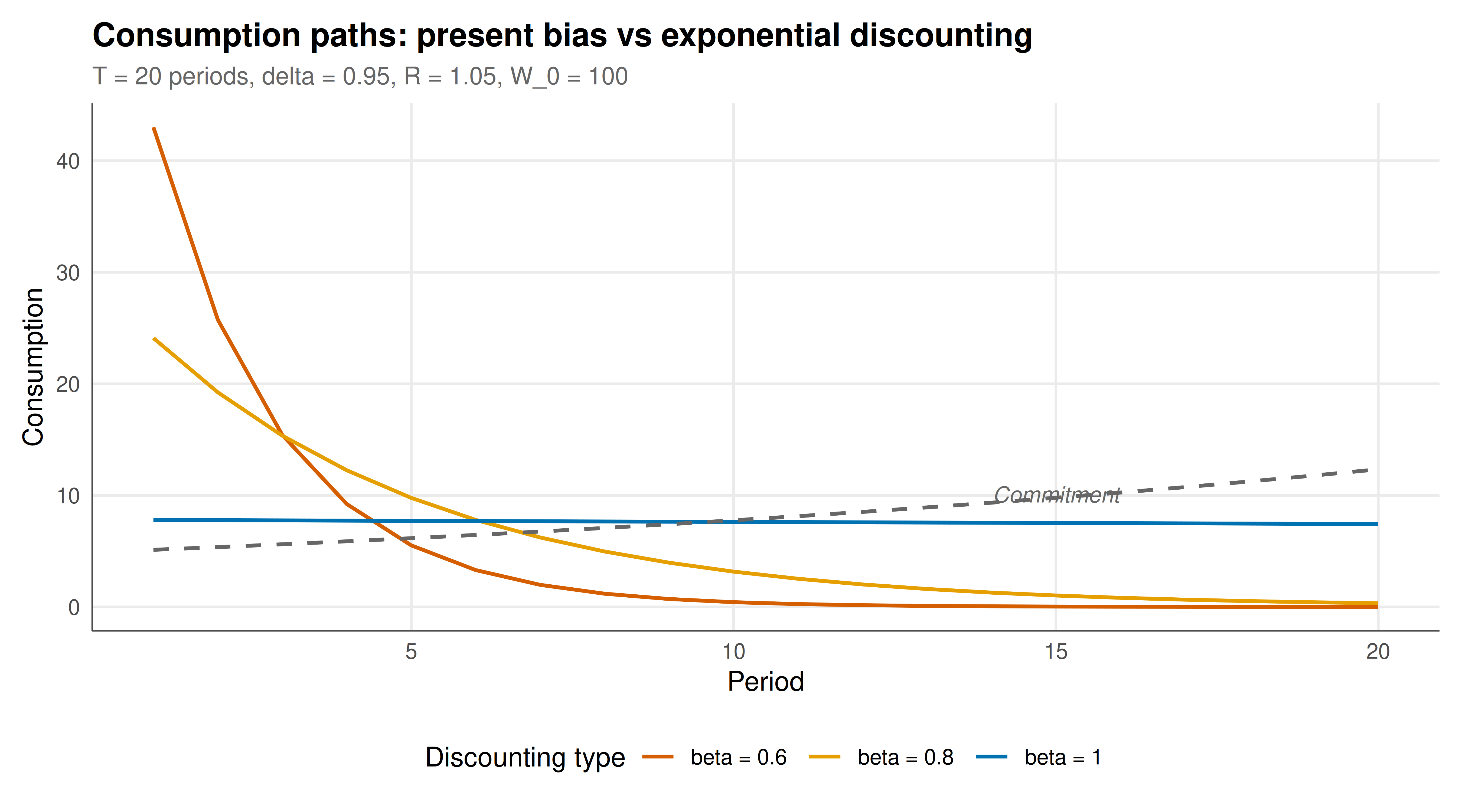
#| fig-cap: "Figure 1. Consumption paths under Markov perfect equilibrium for different levels of present bias. Present-biased agents (beta < 1) front-load consumption relative to exponential discounters (beta = 1), depleting wealth faster. The dashed line shows the commitment solution, which all types would prefer ex ante. Okabe-Ito palette."
#| dev: [png, pdf]
#| fig-width: 9
#| fig-height: 5
#| dpi: 300
commit_plot <- commit_df |>
  mutate(beta_label = "Commitment (delta only)")

consumption_plot <- results_df |>
  select(period, consumption, beta_label)

p_consumption <- ggplot() +
  geom_line(data = consumption_plot,
            aes(x = period, y = consumption, color = beta_label),
            linewidth = 0.8) +
  geom_line(data = commit_plot,
            aes(x = period, y = consumption),
            linewidth = 0.8, linetype = "dashed", color = "grey40") +
  scale_color_manual(values = c("beta = 1" = okabe_ito[5],
                                 "beta = 0.8" = okabe_ito[1],
                                 "beta = 0.6" = okabe_ito[6])) +
  annotate("text", x = 15, y = commit_plot$consumption[15] + 0.3,
           label = "Commitment", color = "grey40", size = 3.5, fontface = "italic") +
  labs(
    title = "Consumption paths: present bias vs exponential discounting",
    subtitle = sprintf("T = %d periods, delta = %.2f, R = %.2f, W_0 = %d",
                       T_horizon, delta, R_return, W_init),
    x = "Period", y = "Consumption",
    color = "Discounting type"
  ) +
  theme_publication()

p_consumption
```
## Interactive figure
```{r}
#| label: fig-cooperation-interactive
coop_plot <- coop_data |>
  mutate(
    text = sprintf("delta = %.2f, beta = %.1f\nRequired patience: %.3f\nCan cooperate: %s",
                   delta, beta, required_patience,
                   ifelse(can_cooperate, "Yes", "No"))
  )

p_coop <- ggplot(coop_plot,
       aes(x = delta, y = beta, fill = can_cooperate, text = text)) +
  geom_tile(width = 0.01, height = 0.05) +
  geom_vline(xintercept = delta_crit_exp, linetype = "dashed",
             color = "white", linewidth = 0.5) +
  scale_fill_manual(values = c("TRUE" = okabe_ito[3], "FALSE" = okabe_ito[6]),
                    labels = c("TRUE" = "Cooperation sustained",
                               "FALSE" = "Defection")) +
  labs(
    title = "Cooperation in repeated PD with hyperbolic discounters",
    subtitle = sprintf("Grim trigger; T=%d, R=%d, P=%d, S=%d; dashed = exponential threshold",
                       T_pd, R_pd, P_pd, S_pd),
    x = expression(paste("Long-run discount factor ", delta)),
    y = expression(paste("Present-bias parameter ", beta)),
    fill = "Outcome"
  ) +
  theme_publication()

ggplotly(p_coop, tooltip = "text") |>
  config(displaylogo = FALSE,
         modeBarButtonsToRemove = c("select2d", "lasso2d"))
```
## Interpretation
The results of our analysis paint a vivid picture of how present bias distorts both individual decision-making and strategic interaction. In the savings game, the Markov perfect equilibrium reveals a systematic pattern: present-biased agents consume too much in early periods and too little in late periods, relative to what they themselves would choose if they could commit. The consumption path for $\beta = 0.6$ (strong present bias) is dramatically front-loaded — the agent devours a large share of wealth immediately, leaving far less for future consumption. With $\beta = 1$ (no present bias), the consumption path closely tracks the commitment solution, as expected: an exponential discounter has no self-control problem and no need for commitment. For intermediate values like $\beta = 0.8$, the distortion is moderate but still economically significant.
The welfare analysis quantifies the cost of present bias. From the perspective of the initial self (period 1), the commitment solution is always weakly preferred to the MPE for any $\beta \leq 1$. The difference — the "value of commitment" — measures how much the agent would be willing to pay for a mechanism that binds her future choices. For $\beta = 0.6$, this value is substantial: the agent would accept a significant reduction in flexibility in exchange for commitment. This result provides the theoretical foundation for understanding why people voluntarily adopt commitment devices such as automatic savings plans, deposit contracts (as studied by Ashraf, Karlan, and Yin, 2006), and self-imposed deadlines. The demand for commitment is not irrational — it is the rational response of a sophisticated present-biased agent who understands her own future weakness.
The intrapersonal game perspective also sheds light on an important distinction in the behavioural economics literature: the difference between naive and sophisticated present-biased agents. A naive agent incorrectly believes that her future selves will not be present-biased (she thinks $\beta_{\text{future}} = 1$), so she makes plans that she will later fail to follow through on. A sophisticated agent correctly predicts her future behaviour and optimises accordingly — this is the MPE we computed. The sophisticated agent consumes more in the first period than the naive agent plans to (because the naive agent's plans are not credible), but less than the naive agent actually ends up consuming (because the naive agent repeatedly procrastinates and over-consumes). In our implementation, we focus on the sophisticated case; the naive case would use different backward induction logic where each self solves as if future selves were time-consistent.
The repeated Prisoner's Dilemma analysis reveals that present bias undermines cooperation in multi-player settings, not just in intrapersonal ones. The grim trigger strategy sustains cooperation in a standard repeated PD when the discount factor $\delta$ exceeds a critical threshold. With present bias, the effective discount factor for the current period's deviation incentive is $\beta \delta$, not $\delta$. Since $\beta < 1$, the cooperation region in $(\delta, \beta)$ space shrinks: combinations of $\delta$ and $\beta$ that would sustain cooperation under exponential discounting fail to do so under quasi-hyperbolic preferences. The heatmap makes this visually clear — the cooperation region is a triangle in $(\delta, \beta)$ space, and more severe present bias ($\beta$ closer to 0) requires correspondingly higher $\delta$ to sustain cooperation. This result has implications for understanding why cooperation often breaks down in practice even when the folk theorem would predict it is sustainable: if agents are present-biased, the effective patience required for cooperation is higher than standard theory suggests.
The broader implications extend to institutional design and public policy. If people are present-biased, then institutions that provide commitment — pensions, contracts, laws — can improve welfare even when they restrict freedom. This is the core argument for "libertarian paternalism" and the broader nudge programme. Our analysis provides the formal game-theoretic foundation for these arguments by modelling the intrapersonal conflict as a well-defined game and computing the welfare gains from resolving it.
## Extensions & related tutorials
- [Prospect theory and reference dependence](../../decision-theory/prospect-theory-reference-dependence/) — another major departure from expected utility theory, focusing on loss aversion rather than time inconsistency.
- [Nudge and libertarian paternalism](../nudge-libertarian-paternalism/) — policy applications of behavioural insights, including commitment device design.
- [Mental accounting and Thaler](../mental-accounting-thaler/) — how people categorise and evaluate financial outcomes in behaviourally realistic ways.
- [Repeated Prisoner's Dilemma and folk theorems](../../classical-games/) — the classical theory of repeated games that hyperbolic discounting modifies.
- [Prospect theory and Kahneman-Tversky](../prospect-theory-kahneman-tversky/) — the foundational behavioural model combining loss aversion, probability weighting, and reference dependence.
## References
::: {#refs}
:::