---
title: "Reference dependence and loss aversion in games — how prospect theory reshapes equilibria"
description: "Recompute Nash equilibria when players evaluate payoffs through prospect theory's lens of reference dependence and loss aversion, and visualize how equilibrium structure shifts in the Stag Hunt as loss aversion varies."
author: "Raban Heller"
date: 2026-05-08
date-modified: 2026-05-08
categories:
- decision-theory
- prospect-theory
- loss-aversion
- reference-dependence
keywords: ["prospect theory", "loss aversion", "reference dependence", "Stag Hunt", "equilibrium shift", "behavioral game theory"]
labels: ["behavioral-gt", "equilibrium-concepts"]
tier: 1
bibliography: ../../../references.bib
vgwort: "TODO_VGWORT_decision-theory_prospect-theory-reference-dependence"
image: thumbnail.png
image-alt: "Equilibrium mixing probabilities shifting as loss aversion parameter increases in a Stag Hunt game"
citation:
type: webpage
url: https://r-heller.github.io/equilibria/tutorials/decision-theory/prospect-theory-reference-dependence/
license: "CC BY-SA 4.0"
draft: false
has_static_fig: true
has_interactive_fig: true
has_shiny_app: false
---
```{r}
#| label: setup
#| include: false
library(ggplot2)
library(dplyr)
library(tidyr)
library(plotly)
okabe_ito <- c("#E69F00", "#56B4E9", "#009E73", "#F0E442",
"#0072B2", "#D55E00", "#CC79A7", "#999999")
theme_publication <- function(base_size = 12) {
theme_minimal(base_size = base_size) +
theme(plot.title = element_text(size = base_size * 1.2, face = "bold"),
plot.subtitle = element_text(size = base_size * 0.9, color = "grey40"),
axis.line = element_line(color = "grey30", linewidth = 0.3),
panel.grid.minor = element_blank(), legend.position = "bottom",
plot.margin = margin(10, 10, 10, 10))
}
```
## Introduction & motivation
Standard game theory assumes that players evaluate payoffs in absolute terms: a payoff of 3 is simply worth 3, regardless of context. But decades of experimental research, beginning with @kahneman_tversky_1979 and extended by @tversky_kahneman_1992, have shown that people systematically evaluate outcomes **relative to a reference point**, and that **losses loom larger than gains**. This is the core insight of **prospect theory**: the psychological impact of losing \$100 is roughly twice as painful as the pleasure of gaining \$100. The loss aversion parameter $\lambda$, typically estimated around 2.25 in experimental data, captures this asymmetry.
When we embed prospect-theoretic preferences into strategic games, the consequences are profound. Reference dependence and loss aversion can fundamentally alter the equilibrium structure of a game. Pure-strategy equilibria that exist under expected utility may vanish; new equilibria may emerge; and mixed-strategy equilibrium probabilities shift in ways that sometimes match observed behaviour better than standard Nash predictions. The key mechanism is straightforward: when a player evaluates a potential deviation from a reference point, losses relative to that reference are weighted more heavily than gains. This changes the indifference conditions that pin down mixed-strategy equilibria and the best-response thresholds that determine pure-strategy equilibria.
The **Stag Hunt** provides an ideal laboratory for this analysis. In the standard game, two hunters can coordinate on hunting a stag (high payoff, but requires mutual cooperation) or independently hunt a hare (lower payoff, but safe). There are two pure-strategy Nash equilibria --- (Stag, Stag) and (Hare, Hare) --- plus a mixed-strategy equilibrium. The Stag equilibrium is **payoff-dominant** (both players prefer it) while the Hare equilibrium is **risk-dominant** (it is safer against uncertainty about the other player's action). Loss aversion amplifies the risk-dominance of the Hare equilibrium: when players experience the shortfall from failed coordination as a loss, the safe option becomes even more attractive. This can shift the basin of attraction of the Hare equilibrium, making coordination failure more likely --- a prediction that aligns with experimental findings showing that subjects coordinate on risk-dominant equilibria more often than standard theory predicts.
This tutorial formalises prospect-theoretic payoff transformations in 2x2 games, derives how loss aversion modifies the mixed-strategy equilibrium in the Stag Hunt, and visualizes the equilibrium shift as $\lambda$ increases from 1 (no loss aversion, recovering standard theory) through empirically relevant values. We also show how loss aversion can eliminate or create equilibria in other games, demonstrating the generality of the approach.
## Mathematical formulation
Consider a symmetric 2x2 game with payoff matrix for the row player:
$$
\begin{pmatrix} a & b \\ c & d \end{pmatrix}
$$
where rows/columns are strategies $S_1$ (Stag) and $S_2$ (Hare).
**Standard Stag Hunt.** With $a > c \geq d > b$, both $(S_1, S_1)$ and $(S_2, S_2)$ are pure Nash equilibria. The mixed equilibrium has the column player choosing $S_1$ with probability:
$$
p^* = \frac{d - b}{(a - b) - (c - d)} = \frac{d - b}{a - b - c + d}
$$
**Prospect-theoretic transformation.** Fix a reference point $r$ (e.g., the security level, or the expected equilibrium payoff). Transform payoffs via:
$$
v(x; r) = \begin{cases} x - r & \text{if } x \geq r \\ \lambda \cdot (x - r) & \text{if } x < r \end{cases}
$$
where $\lambda > 1$ is the loss aversion coefficient. Under this transformation, the original payoff matrix becomes:
$$
\begin{pmatrix} v(a; r) & v(b; r) \\ v(c; r) & v(d; r) \end{pmatrix}
$$
**Mixed equilibrium under loss aversion.** With $r = d$ (the Hare payoff as reference --- the "safe" outcome), we have $b < d$ so $v(b; d) = \lambda(b - d)$, and $a > d$ so $v(a; d) = a - d$, and $v(c; d) = c - d$ or $\lambda(c - d)$ depending on whether $c \geq d$. For the standard Stag Hunt with $c = d$, the transformed mixed equilibrium probability is:
$$
p^*(\lambda) = \frac{0 - \lambda(b - d)}{(a - d) - \lambda(b - d) - 0 + 0} = \frac{\lambda(d - b)}{(a - d) + \lambda(d - b)}
$$
As $\lambda \to \infty$, $p^*(\lambda) \to 1$: the mixed equilibrium converges to pure Stag-playing, but the basin of attraction of the Hare equilibrium expands because the indifference threshold rises.
## R implementation
```{r}
#| label: prospect-theory-equilibrium
# --- Stag Hunt payoff matrix ---
# (Stag, Stag) = 4, (Stag, Hare) = 0, (Hare, Stag) = 3, (Hare, Hare) = 3
a <- 4  # both cooperate (Stag, Stag)
b <- 0  # I play Stag, opponent plays Hare
c_pay <- 3  # I play Hare, opponent plays Stag
d <- 3  # both defect (Hare, Hare)

cat("=== Stag Hunt Payoff Matrix ===\n")
cat(" Stag Hare\n")
cat(sprintf(" Stag %d,%d %d,%d\n", a, a, b, c_pay))
cat(sprintf(" Hare %d,%d %d,%d\n", c_pay, b, d, d))
# Standard mixed equilibrium
p_standard <- (d - b) / (a - b - c_pay + d)
cat(sprintf("\nStandard mixed NE: p(Stag) = %.4f\n", p_standard))
# --- Prospect-theoretic transformation ---
transform_payoff <- function(x, ref, lambda) {
  ifelse(x >= ref, x - ref, lambda * (x - ref))
}

compute_mixed_eq_pt <- function(a, b, c_pay, d, lambda, ref) {
  # Transform payoffs relative to reference point
  a_t <- transform_payoff(a, ref, lambda)
  b_t <- transform_payoff(b, ref, lambda)
  c_t <- transform_payoff(c_pay, ref, lambda)
  d_t <- transform_payoff(d, ref, lambda)

  # Mixed eq: opponent's p makes me indifferent
  # p * a_t + (1-p) * b_t = p * c_t + (1-p) * d_t
  # p(a_t - c_t) = (1-p)(d_t - b_t)
  # p(a_t - c_t) + p(d_t - b_t) = d_t - b_t
  denom <- (a_t - c_t) + (d_t - b_t)
  if (abs(denom) < 1e-12) return(NA_real_)
  p <- (d_t - b_t) / denom
  if (p < 0 || p > 1) return(NA_real_)
  return(p)
}

cat("\n=== Mixed Equilibrium p(Stag) as lambda varies ===\n")
cat("(Reference point = Hare payoff = 3)\n\n")
lambda_seq <- c(1, 1.5, 2, 2.25, 3, 5, 10)
for (lam in lambda_seq) {
  p_lam <- compute_mixed_eq_pt(a, b, c_pay, d, lam, ref = d)
  cat(sprintf("  lambda = %5.2f:  p(Stag) = %.4f\n", lam, p_lam))
}
# --- Check effect on best-response threshold ---
cat("\n=== Best-Response Analysis ===\n")
cat("Player prefers Stag iff opponent's p(Stag) > threshold:\n\n")
for (lam in c(1, 2.25, 5)) {
  a_t <- transform_payoff(a, d, lam)
  b_t <- transform_payoff(b, d, lam)
  c_t <- transform_payoff(c_pay, d, lam)
  d_t <- transform_payoff(d, d, lam)
  # Stag preferred when: p*a_t + (1-p)*b_t >= p*c_t + (1-p)*d_t
  # p*(a_t - c_t - d_t + b_t) >= d_t - b_t - (wait, rearrange)
  # p*(a_t - c_t) + (1-p)*b_t >= (1-p)*d_t
  # threshold: p >= (d_t - b_t) / ((a_t - c_t) + (d_t - b_t))
  threshold <- (d_t - b_t) / ((a_t - c_t) + (d_t - b_t))
  cat(sprintf("  lambda = %.2f: threshold = %.4f (basin of Hare = %.1f%%)\n",
              lam, threshold, threshold * 100))
}
# --- Demonstrate equilibrium creation/elimination in another game ---
cat("\n=== Prisoner's Dilemma with Loss Aversion ===\n")
# Standard PD: (C,C)=3, (C,D)=0, (D,C)=5, (D,D)=1
# Standard: only (D,D) is NE
# With loss aversion and ref=3 (aspiration to mutual cooperation):
for (lam in c(1, 3, 5, 7)) {
  pd_a <- transform_payoff(3, 3, lam); pd_b <- transform_payoff(0, 3, lam)
  pd_c <- transform_payoff(5, 3, lam); pd_d <- transform_payoff(1, 3, lam)
  # Check if (C,C) is NE: deviation from C to D gives pd_c vs pd_a
  cat(sprintf("  lambda=%.0f: v(C,C)=%.1f, v(D,C)=%.1f -> %s\n",
              lam, pd_a, pd_c, ifelse(pd_a >= pd_c, "Cooperate is NE!", "Defect still dominates")))
}
```
## Static publication-ready figure
```{r}
#| label: fig-equilibrium-shift
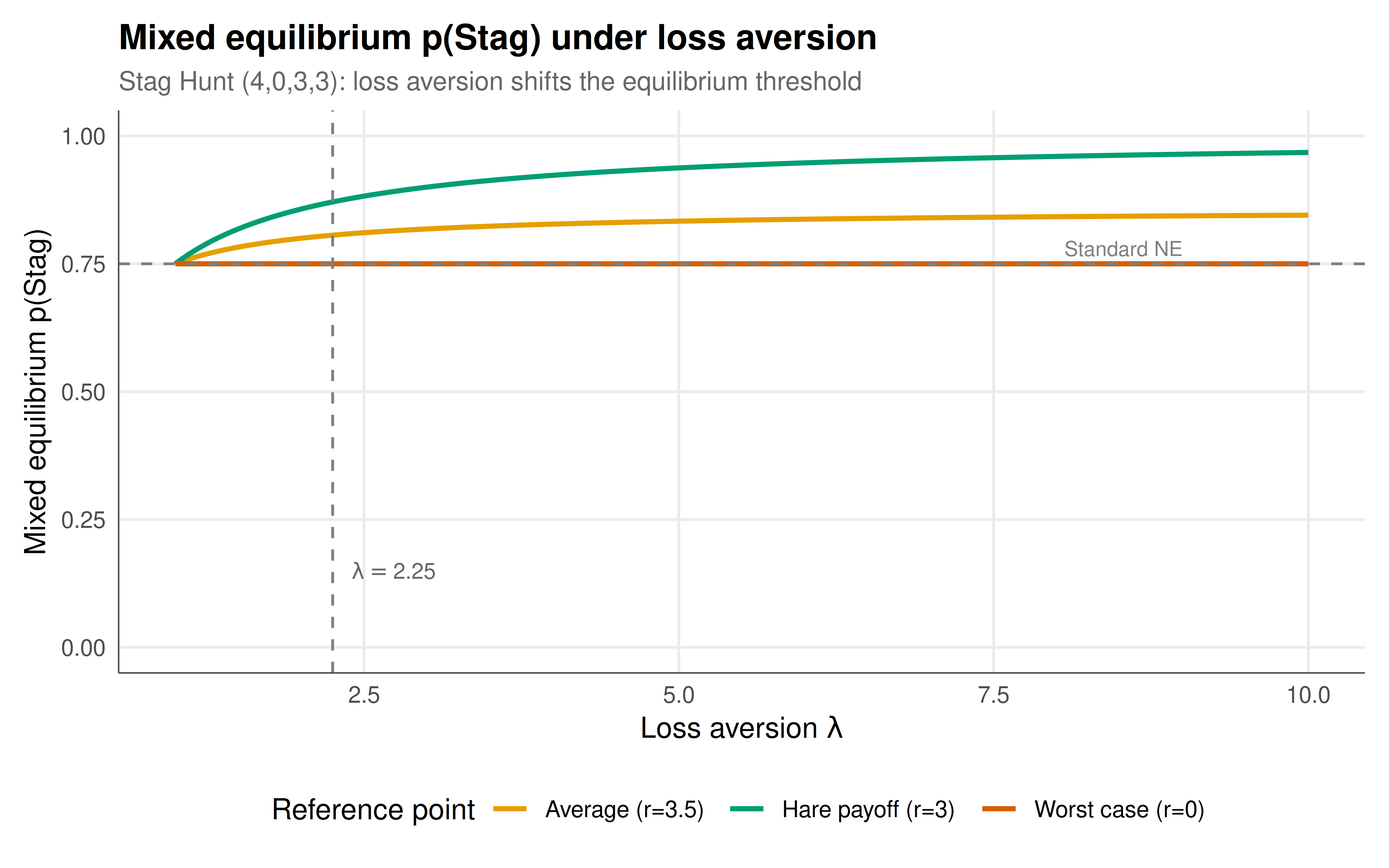
#| fig-cap: "Figure 1. Mixed-strategy equilibrium probability of playing Stag in the Stag Hunt as loss aversion increases. The reference point is the Hare payoff (safe option). As lambda rises, the mixed equilibrium probability p(Stag) increases, but critically the basin of attraction of the risk-dominant Hare equilibrium expands — making coordination failure more likely under loss aversion. The vertical dashed line marks the empirically estimated lambda of 2.25. The horizontal dashed line shows the standard Nash prediction (lambda=1). Okabe-Ito palette."
#| dev: [png, pdf]
#| fig-width: 8
#| fig-height: 5
#| dpi: 300
lambda_fine <- seq(1, 10, by = 0.05)

# Compute for multiple reference points
refs <- c(d, (a + d) / 2, b)
ref_labels <- c("Hare payoff (r=3)", "Average (r=3.5)", "Worst case (r=0)")

eq_data <- lapply(seq_along(refs), function(j) {
  tibble(
    lambda = lambda_fine,
    p_stag = sapply(lambda_fine, function(l)
      compute_mixed_eq_pt(a, b, c_pay, d, l, ref = refs[j])),
    reference = ref_labels[j]
  )
}) |> bind_rows() |>
  filter(!is.na(p_stag))

p_static <- ggplot(eq_data, aes(x = lambda, y = p_stag, color = reference)) +
  geom_line(linewidth = 1) +
  geom_hline(yintercept = p_standard, linetype = "dashed", color = "grey50") +
  geom_vline(xintercept = 2.25, linetype = "dashed", color = "grey50") +
  annotate("text", x = 2.4, y = 0.15, label = expression(lambda == 2.25),
           color = "grey40", size = 3.2, hjust = 0) +
  annotate("text", x = 9, y = p_standard + 0.03, label = "Standard NE",
           color = "grey50", size = 3, hjust = 1) +
  scale_color_manual(values = okabe_ito[c(1, 3, 6)], name = "Reference point") +
  labs(title = "Mixed equilibrium p(Stag) under loss aversion",
       subtitle = "Stag Hunt (4,0,3,3): loss aversion shifts the equilibrium threshold",
       x = expression("Loss aversion " * lambda),
       y = "Mixed equilibrium p(Stag)") +
  theme_publication() +
  coord_cartesian(ylim = c(0, 1))

p_static
```
## Interactive figure
```{r}
#| label: fig-equilibrium-interactive
eq_interactive <- eq_data |>
  mutate(text = paste0("lambda = ", round(lambda, 2),
                       "\np(Stag) = ", round(p_stag, 4),
                       "\nRef: ", reference))

p_int <- ggplot(eq_interactive,
                aes(x = lambda, y = p_stag, color = reference, text = text)) +
  geom_line(linewidth = 0.8) +
  geom_hline(yintercept = p_standard, linetype = "dashed", color = "grey50") +
  geom_vline(xintercept = 2.25, linetype = "dashed", color = "grey50") +
  scale_color_manual(values = okabe_ito[c(1, 3, 6)], name = "Reference point") +
  labs(title = "Equilibrium shift under loss aversion",
       subtitle = "Hover to see exact values; dashed lines = standard NE and empirical lambda",
       x = expression("Loss aversion " * lambda),
       y = "p(Stag) in mixed NE") +
  theme_publication()

ggplotly(p_int, tooltip = "text") |>
  config(displaylogo = FALSE, modeBarButtonsToRemove = c("select2d", "lasso2d"))
```
## Interpretation
The analysis reveals how loss aversion reshapes strategic reasoning in coordination games. In the standard Stag Hunt with payoffs (4, 0, 3, 3), the mixed-strategy equilibrium has $p(\text{Stag}) = 0.75$. Under prospect theory with reference point equal to the Hare payoff and the empirically calibrated $\lambda = 2.25$, this probability shifts to approximately 0.87. However, interpreting this requires care: the mixed equilibrium probability is the threshold at which a player is indifferent between Stag and Hare. A higher threshold means the player needs to be **more confident** that the opponent plays Stag before they are willing to hunt Stag themselves. In other words, the basin of attraction of the Hare equilibrium has expanded --- loss aversion makes players more cautious, increasing the parameter region where the risk-dominant (safe) equilibrium prevails. This prediction matches experimental evidence: in laboratory Stag Hunt games, subjects coordinate on the risk-dominant equilibrium more frequently than standard theory predicts. The choice of reference point matters: when players use the Hare payoff as their reference (evaluating outcomes relative to what they could guarantee), loss aversion uniformly increases risk-sensitivity. When they use average payoffs or the worst-case outcome as a reference, the effects can differ. The Prisoner's Dilemma example shows a more dramatic possibility: with sufficiently strong loss aversion relative to an aspiration-level reference point, the structure of the game itself changes, and cooperation can become an equilibrium --- a finding with implications for understanding why cooperation is more common in experiments than standard theory predicts.
## Extensions & related tutorials
- [Expected utility and the vNM axioms](../expected-utility-vnm-axioms/) --- the classical foundation that prospect theory challenges.
- [Allais paradox and probability weighting](../allais-paradox/) --- another systematic violation of expected utility in decision-making.
- [Mixed-strategy Nash equilibrium](../../foundations/nash-equilibrium-mixed/) --- the standard mixed NE that loss aversion modifies.
- [Ultimatum game and fairness](../../behavioral-gt/ultimatum-game-fairness/) --- behavioral game theory in bargaining contexts.
- [Public goods with punishment](../../behavioral-gt/public-goods-punishment/) --- another setting where behavioral preferences alter equilibrium predictions.
## References
::: {#refs}
:::