Expected utility theory and the von Neumann–Morgenstern axioms

Derive expected utility from the VNM axioms in R, demonstrate the representation theorem with numerical examples, and visualize risk attitudes through utility function curvature.

Keywords

expected utility, von Neumann-Morgenstern, axioms, risk aversion, utility function, lottery

Introduction & motivation

Expected utility theory is the mathematical bedrock of decision-making under uncertainty — and by extension, of game theory itself. When Nash defined mixed-strategy equilibria, he assumed players maximise expected utility over lotteries induced by mixed strategies. But why should rational agents maximise expected utility rather than, say, expected wealth or median wealth? The answer lies in the axioms of Neumann and Morgenstern (1944): if a decision-maker’s preferences over lotteries satisfy four axioms (completeness, transitivity, continuity, independence), then there exists a utility function \(u\) such that the agent prefers lottery \(L_1\) to \(L_2\) if and only if \(E[u(L_1)] > E[u(L_2)]\). This representation theorem transforms the problem of rational choice under uncertainty from a philosophical question into a mathematical one: specify the utility function, compute expectations, and choose the option with the highest expected utility. The shape of the utility function encodes risk attitudes: concave utility implies risk aversion (preferring a certain outcome to a gamble with the same expected value), convex implies risk-seeking, and linear implies risk-neutrality. This tutorial derives the VNM framework, implements expected utility calculations for arbitrary lotteries, and visualizes how different utility functions produce different choices — laying the foundation for every strategic analysis in game theory.

Mathematical formulation

Let \(X\) be a set of outcomes and \(\mathcal{L}(X)\) the set of lotteries (probability distributions) over \(X\). A preference relation \(\succeq\) on \(\mathcal{L}(X)\) satisfies the VNM axioms if:

1. Completeness: For any \(L_1, L_2 \in \mathcal{L}\), either \(L_1 \succeq L_2\) or \(L_2 \succeq L_1\).
2. Transitivity: \(L_1 \succeq L_2\) and \(L_2 \succeq L_3\) implies \(L_1 \succeq L_3\).
3. Continuity: If \(L_1 \succ L_2 \succ L_3\), there exists \(\alpha \in (0,1)\) such that \(L_2 \sim \alpha L_1 + (1-\alpha) L_3\).
4. Independence: \(L_1 \succ L_2\) implies \(\alpha L_1 + (1-\alpha) L_3 \succ \alpha L_2 + (1-\alpha) L_3\) for all \(\alpha \in (0,1)\) and all \(L_3\).

Theorem (VNM): \(\succeq\) satisfies axioms 1–4 if and only if there exists \(u: X \to \mathbb{R}\) such that \(L_1 \succeq L_2 \iff E_L[u(L_1)] \geq E_L[u(L_2)]\).

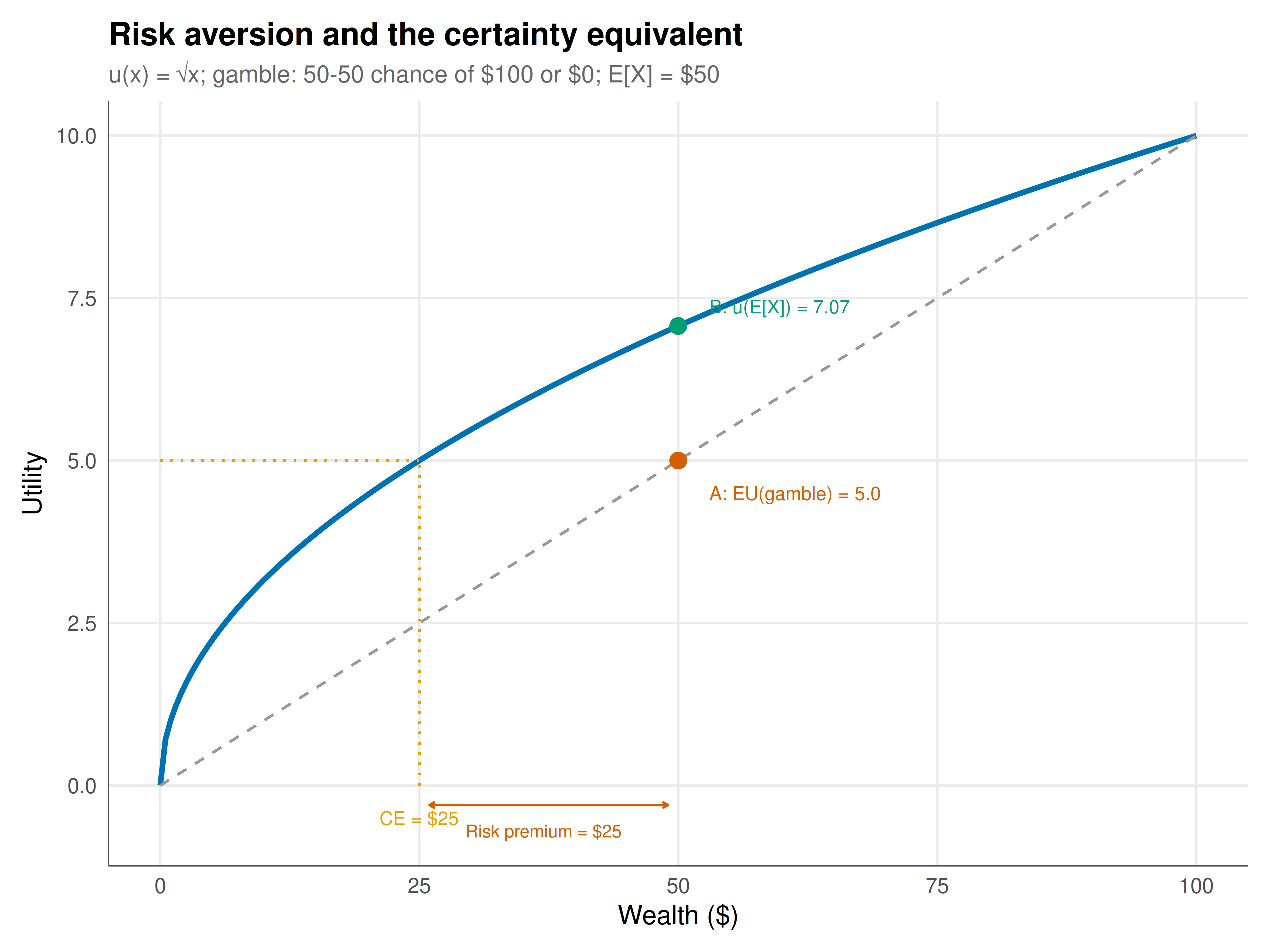
Risk aversion: An agent is risk-averse if \(u\) is concave: \(u(E[X]) > E[u(X)]\) for any non-degenerate lottery. The certainty equivalent \(CE\) satisfies \(u(CE) = E[u(X)]\), and the risk premium is \(\pi = E[X] - CE\).

R implementation

# Expected utility calculator
expected_utility <- function(outcomes, probs, utility_fn) {
  sum(probs * utility_fn(outcomes))
}

# Common utility functions
u_risk_neutral <- function(x) x
u_risk_averse <- function(x) sqrt(x)  # concave
u_risk_seeking <- function(x) x^2      # convex
u_log <- function(x) log(x + 1)        # strongly risk-averse

# --- Decision example: fair coin flip ---
# Lottery A: 50% chance of $100, 50% chance of $0
# Lottery B: $50 for certain
outcomes_A <- c(100, 0)
probs_A <- c(0.5, 0.5)
outcomes_B <- c(50)
probs_B <- c(1)

cat("=== Fair gamble: 50-50 chance of $100 or $0 vs certain $50 ===\n\n")

=== Fair gamble: 50-50 chance of $100 or $0 vs certain $50 ===

utility_fns <- list(
  "Risk-neutral (u=x)" = u_risk_neutral,
  "Risk-averse (u=√x)" = u_risk_averse,
  "Risk-seeking (u=x²)" = u_risk_seeking,
  "Log utility (u=ln(x+1))" = u_log
)

for (name in names(utility_fns)) {
  fn <- utility_fns[[name]]
  eu_A <- expected_utility(outcomes_A, probs_A, fn)
  eu_B <- expected_utility(outcomes_B, probs_B, fn)
  choice <- ifelse(eu_A > eu_B, "Gamble", ifelse(eu_A < eu_B, "Certain $50", "Indifferent"))
  cat(sprintf("  %s: EU(gamble)=%.2f, EU(certain)=%.2f → %s\n",
              name, eu_A, eu_B, choice))
}

  Risk-neutral (u=x): EU(gamble)=50.00, EU(certain)=50.00 → Indifferent
  Risk-averse (u=√x): EU(gamble)=5.00, EU(certain)=7.07 → Certain $50
  Risk-seeking (u=x²): EU(gamble)=5000.00, EU(certain)=2500.00 → Gamble
  Log utility (u=ln(x+1)): EU(gamble)=2.31, EU(certain)=3.93 → Certain $50

# Certainty equivalent for risk-averse agent
ce_sqrt <- (expected_utility(outcomes_A, probs_A, u_risk_averse))^2
risk_premium <- 50 - ce_sqrt
cat(sprintf("\nCertainty equivalent (√x): $%.2f\n", ce_sqrt))

Certainty equivalent (√x): $25.00

cat(sprintf("Risk premium: $%.2f (willing to pay this to avoid gamble)\n", risk_premium))

Risk premium: $25.00 (willing to pay this to avoid gamble)

Static publication-ready figure

x_seq <- seq(0, 100, by = 0.5)

util_df <- tibble(x = rep(x_seq, 3),
                   type = rep(c("Risk-averse (√x)", "Risk-neutral (x)", "Risk-seeking (x²)"),
                              each = length(x_seq)),
                   utility = c(sqrt(x_seq), x_seq / 10, x_seq^2 / 10000 * 10))

# Normalise for visual comparison
util_df <- tibble(x = rep(x_seq, 3),
                   type = rep(c("Risk-averse: u = √x", "Risk-neutral: u = x/10", "Risk-seeking: u = x²/1000"),
                              each = length(x_seq)),
                   utility = c(sqrt(x_seq), x_seq / 10, x_seq^2 / 1000))

# Focus on risk-averse case for annotation
ra_df <- tibble(x = x_seq, u = sqrt(x_seq))

# Key points for gamble illustration
eu_gamble <- 0.5 * sqrt(100) + 0.5 * sqrt(0)  # = 5
u_certain <- sqrt(50)  # ≈ 7.07
ce <- eu_gamble^2  # = 25

p_util <- ggplot(ra_df, aes(x = x, y = u)) +
  geom_line(color = okabe_ito[5], linewidth = 1.2) +
  # Chord from (0,0) to (100,10)
  geom_segment(aes(x = 0, y = 0, xend = 100, yend = 10),
               linetype = "dashed", color = "grey60") +
  # Expected value point on chord
  geom_point(aes(x = 50, y = 5), color = okabe_ito[6], size = 3) +
  annotate("text", x = 53, y = 4.5, label = "A: EU(gamble) = 5.0",
           size = 3, color = okabe_ito[6], hjust = 0) +
  # Utility of certain EV
  geom_point(aes(x = 50, y = u_certain), color = okabe_ito[3], size = 3) +
  annotate("text", x = 53, y = u_certain + 0.3, label = sprintf("B: u(E[X]) = %.2f", u_certain),
           size = 3, color = okabe_ito[3], hjust = 0) +
  # Certainty equivalent
  geom_segment(aes(x = ce, y = 0, xend = ce, yend = eu_gamble),
               linetype = "dotted", color = okabe_ito[1]) +
  geom_segment(aes(x = 0, y = eu_gamble, xend = ce, yend = eu_gamble),
               linetype = "dotted", color = okabe_ito[1]) +
  annotate("text", x = ce, y = -0.5, label = sprintf("CE = $%.0f", ce),
           size = 3, color = okabe_ito[1]) +
  # Risk premium bracket
  annotate("segment", x = ce + 1, y = -0.3, xend = 49, yend = -0.3,
           arrow = arrow(ends = "both", length = unit(0.1, "cm")), color = okabe_ito[6]) +
  annotate("text", x = 37, y = -0.7, label = sprintf("Risk premium = $%.0f", 50 - ce),
           size = 2.8, color = okabe_ito[6]) +
  labs(
    title = "Risk aversion and the certainty equivalent",
    subtitle = "u(x) = √x; gamble: 50-50 chance of $100 or $0; E[X] = $50",
    x = "Wealth ($)", y = "Utility"
  ) +
  theme_publication()

p_util

Figure 1: Figure 1. Three utility functions and risk attitudes. Concave utility (√x, blue) implies risk aversion: the expected utility of a fair gamble (point A) lies below the utility of the certain expected value (point B), so the agent prefers the sure thing. The certainty equivalent CE is the guaranteed amount giving the same utility as the gamble. Convex utility (x², red) implies risk-seeking: the agent prefers the gamble. Linear utility (x, grey) is risk-neutral. Okabe-Ito palette.

Interactive figure

# Risk premium as a function of wealth level for different utility functions
wealth_seq <- seq(10, 200, by = 5)
gamble_size <- 50  # ±$50 fair gamble

rp_data <- tibble(wealth = rep(wealth_seq, 2),
                   type = rep(c("√x (moderate risk aversion)", "ln(x+1) (strong risk aversion)"),
                              each = length(wealth_seq))) |>
  rowwise() |>
  mutate(
    eu = ifelse(grepl("√", type),
                0.5 * sqrt(wealth + gamble_size) + 0.5 * sqrt(max(0.01, wealth - gamble_size)),
                0.5 * log(wealth + gamble_size + 1) + 0.5 * log(max(0.01, wealth - gamble_size) + 1)),
    ce = ifelse(grepl("√", type), eu^2, exp(eu) - 1),
    risk_premium = wealth - ce,
    text = paste0("Wealth: $", wealth, "\nType: ", type,
                  "\nCE: $", round(ce, 1), "\nRisk premium: $", round(risk_premium, 1))
  ) |>
  ungroup()

p_rp <- ggplot(rp_data, aes(x = wealth, y = risk_premium, color = type, text = text)) +
  geom_line(linewidth = 1) +
  scale_color_manual(values = c(okabe_ito[5], okabe_ito[6]), name = "Utility function") +
  labs(
    title = "Risk premium vs wealth for a ±$50 fair gamble",
    subtitle = "Risk premium decreases with wealth (DARA) for both utility functions",
    x = "Initial wealth ($)", y = "Risk premium ($)"
  ) +
  theme_publication()

ggplotly(p_rp, tooltip = "text") |>
  config(displaylogo = FALSE,
         modeBarButtonsToRemove = c("select2d", "lasso2d"))

Figure 2

Interpretation

Expected utility theory provides the rational foundation for all strategic analysis under uncertainty. The VNM representation theorem shows that four simple axioms — each individually compelling — are sufficient to imply that rational agents act as if they are maximising a weighted sum of utilities. The practical power lies in the utility function: once specified, it determines all choices, risk attitudes, and certainty equivalents. The risk-averse agent (concave \(u\)) is the empirically dominant case: most people prefer $50 for certain over a 50-50 gamble between $100 and $0, revealing that the psychological cost of losing exceeds the psychological benefit of winning. The risk premium quantifies this — for \(u(x) = \sqrt{x}\), an agent would accept as little as $25 for certain instead of the $50-expected-value gamble. This matters profoundly for game theory: in mixed-strategy equilibria, players must be willing to randomise, which requires indifference between pure strategies at the equilibrium mixing probabilities — a condition that depends on the shape of \(u\). The interactive analysis reveals that risk premiums typically decrease with wealth (decreasing absolute risk aversion, DARA), explaining why wealthy individuals accept larger gambles. Expected utility is not the final word — prospect theory, rank-dependent utility, and other non-expected utility models capture systematic violations of the VNM axioms — but it remains the benchmark against which all alternatives are measured and the assumed framework in the vast majority of game-theoretic analysis.

Extensions & related tutorials

• Mixed-strategy Nash equilibrium — expected utility applied to strategic interaction.
• Nash bargaining solution — bargaining under risk.
• Prospect theory and behavioural deviations — when VNM axioms fail.
• The Allais paradox — the most famous violation of the independence axiom.
• Mechanism design under risk — designing institutions for risk-averse agents.

References

Neumann, John von, and Oskar Morgenstern. 1944. Theory of Games and Economic Behavior. Princeton University Press.