---
title: "OPEC as a cartel — oligopoly theory applied to oil markets"
description: "Model OPEC as a repeated Cournot oligopoly with heterogeneous producers, compute Nash and cartel equilibria, analyse deviation incentives, and determine the critical discount factor for cartel sustainability."
author: "Raban Heller"
date: 2026-05-08
date-modified: 2026-05-08
categories:
- case-studies
- oligopoly
- cartel
- opec
keywords: ["OPEC", "cartel stability", "Cournot oligopoly", "folk theorem", "trigger strategy"]
labels: ["industrial-organization", "applied-game-theory"]
tier: 1
bibliography: ../../../references.bib
vgwort: "TODO_VGWORT_case-studies_opec-cartel-oligopoly"
image: thumbnail.png
image-alt: "Comparison of competitive Cournot-Nash equilibrium, cartel output, and deviation payoffs for OPEC-style oligopoly"
citation:
type: webpage
url: https://r-heller.github.io/equilibria/tutorials/case-studies/opec-cartel-oligopoly/
license: "CC BY-SA 4.0"
draft: false
has_static_fig: true
has_interactive_fig: true
has_shiny_app: false
---
```{r}
#| label: setup
#| include: false
library(ggplot2)
library(dplyr)
library(tidyr)
library(plotly)
okabe_ito <- c("#E69F00", "#56B4E9", "#009E73", "#F0E442",
"#0072B2", "#D55E00", "#CC79A7", "#999999")
theme_publication <- function(base_size = 12) {
theme_minimal(base_size = base_size) +
theme(plot.title = element_text(size = base_size * 1.2, face = "bold"),
plot.subtitle = element_text(size = base_size * 0.9, color = "grey40"),
axis.line = element_line(color = "grey30", linewidth = 0.3),
panel.grid.minor = element_blank(), legend.position = "bottom",
plot.margin = margin(10, 10, 10, 10))
}
```
## Introduction & motivation
The Organisation of the Petroleum Exporting Countries (OPEC) is arguably the most prominent and consequential cartel in the history of modern economics. Founded in 1960 by five oil-producing nations — Iran, Iraq, Kuwait, Saudi Arabia, and Venezuela — and later expanded to include additional members, OPEC has attempted for more than six decades to coordinate production decisions among sovereign nations to influence world oil prices. The economic stakes are enormous: oil remains the single most traded commodity in the world, and OPEC members collectively control approximately 40% of global oil production and over 70% of proven reserves. OPEC's production decisions affect not only the revenues of member states but also global inflation, economic growth, geopolitical stability, and the pace of the energy transition.
From the perspective of game theory, OPEC presents a fascinating and rich case study in cartel formation and sustainability. A cartel is a group of firms (or, in this case, countries) that agree to restrict output below the competitive level in order to raise prices and increase joint profits. The fundamental challenge facing any cartel is the tension between collective interest and individual incentive: while all members benefit from restricting output collectively, each individual member has a unilateral incentive to cheat on the agreement by producing more than its quota. This is the classic structure of a Prisoner's Dilemma played among oligopolists. If every member cheats, the cartel collapses and prices fall to the competitive level, making everyone worse off. But the temptation to cheat is always present, because a single defector can capture a larger market share at the cartel price — at least until others respond.
The theory of repeated games provides the analytical framework for understanding when cartels can be sustained. In a one-shot Cournot game, the unique Nash equilibrium involves all firms producing at the competitive level — the cartel outcome is not an equilibrium because each firm has a profitable deviation. But when the game is repeated infinitely (or with sufficient probability of continuation), the folk theorem tells us that the cartel outcome can be sustained as a subgame perfect equilibrium using trigger strategies, provided that all members are sufficiently patient. The critical discount factor $\delta^*$ above which cartel cooperation is sustainable depends on the number of members, the demand and cost parameters, and the heterogeneity of producers. The closer $\delta^*$ is to zero, the easier the cartel is to sustain; the closer it is to one, the more precarious the arrangement.
OPEC's history provides rich empirical evidence for these theoretical predictions. The cartel's greatest success was the oil embargo and price increases of 1973-74, when coordinated production cuts quadrupled the world oil price and generated enormous rents for member states. But OPEC has also experienced repeated episodes of quota violations, internal disputes, and price collapses — most notably in 1986, when Saudi Arabia abandoned its role as "swing producer" (absorbing output cuts to maintain prices) and opened the taps, causing prices to crash. More recently, the rise of US shale oil production has complicated OPEC's ability to control prices, leading to the formation of OPEC+ (including Russia and other non-OPEC producers) to coordinate on a larger scale. Each of these episodes can be understood through the lens of repeated game theory: changes in demand, costs, the number of producers, and discount factors shift the critical conditions for cartel sustainability.
In this tutorial, we build a Cournot oligopoly model calibrated to stylised oil market parameters. We compute the competitive (Nash) equilibrium, the cartel (joint profit maximisation) outcome, and the deviation payoffs for each member. We then derive the critical discount factor for sustaining the cartel using grim trigger strategies and analyse how it varies with the number of producers and cost heterogeneity. The simulation includes a realistic feature of oil markets: heterogeneous production costs, reflecting the fact that Saudi Arabia has among the lowest extraction costs in the world, while other OPEC members and non-OPEC producers have significantly higher costs. This heterogeneity has important implications for cartel stability, as low-cost producers have more to gain from deviation and less to lose from punishment.
## Mathematical formulation
**Cournot oligopoly.** There are $n$ producers indexed by $i = 1, \ldots, n$. Producer $i$ chooses output quantity $q_i \geq 0$. Total output is $Q = \sum_{i=1}^n q_i$. The inverse demand function is linear:
$$
P(Q) = a - bQ, \quad a, b > 0
$$
Producer $i$'s cost function is linear: $C_i(q_i) = c_i q_i$, where $c_i$ is the marginal cost. Profit is:
$$
\pi_i(q_i, Q_{-i}) = (P(Q) - c_i) q_i = (a - b(q_i + Q_{-i}) - c_i) q_i
$$
**Cournot-Nash equilibrium.** Each firm maximises profit taking others' outputs as given. The first-order condition for firm $i$:
$$
\frac{\partial \pi_i}{\partial q_i} = a - 2bq_i - bQ_{-i} - c_i = 0
$$
The Nash equilibrium quantities (for $n$ symmetric firms with $c_i = c$):
$$
q_i^N = \frac{a - c}{b(n+1)}, \quad Q^N = \frac{n(a-c)}{b(n+1)}, \quad P^N = \frac{a + nc}{n+1}
$$
**Cartel (joint profit maximisation).** The cartel maximises $\sum_i \pi_i$. For symmetric firms, this yields the monopoly outcome shared equally:
$$
Q^M = \frac{a - c}{2b}, \quad q_i^M = \frac{Q^M}{n}, \quad P^M = \frac{a + c}{2}
$$
**Deviation payoff.** If firm $i$ deviates while others produce $q_j^M$, it chooses the best response to $Q_{-i}^M = (n-1)q_j^M$:
$$
q_i^D = \frac{a - c - b(n-1)q_j^M}{2b} = \frac{(n+1)(a-c)}{4nb}
$$
$$
\pi_i^D = b(q_i^D)^2 = \frac{(n+1)^2(a-c)^2}{16n^2 b}
$$
**Trigger strategy and critical discount factor.** Under a grim trigger strategy, deviation triggers permanent reversion to the Nash equilibrium. The cartel is sustainable if:
$$
\frac{\pi_i^M}{1-\delta} \geq \pi_i^D + \frac{\delta \pi_i^N}{1-\delta}
$$
Solving for $\delta$:
$$
\delta \geq \delta^* = \frac{\pi_i^D - \pi_i^M}{\pi_i^D - \pi_i^N}
$$
For symmetric Cournot with $n$ firms:
$$
\delta^* = \frac{(n+1)^2 - 4n^2/4}{(n+1)^2 - n^2(n+1)^2/(n+1)^2} = \frac{(n+1)^2}{(n+1)^2 + 4n - 4n^2} \text{ (simplified below)}
$$
More precisely, for symmetric firms: $\delta^* = \frac{(n+1)^2}{4n^2 + (n+1)^2 - 4n^2} $. The exact formula depends on proper substitution; we compute it numerically below.
## R implementation
```{r}
#| label: cournot-model
set.seed(42)

# Market parameters (stylised oil market)
a <- 120       # Demand intercept ($/barrel at Q=0)
b <- 0.001     # Demand slope ($/barrel per thousand barrels/day)

# Producers: OPEC members (stylised)
producers <- data.frame(
  name = c("Saudi Arabia", "Iraq", "UAE", "Kuwait", "Iran",
           "Nigeria", "Venezuela", "Non-OPEC fringe"),
  cost = c(10, 15, 12, 10, 18, 25, 30, 35),  # Marginal cost $/barrel
  stringsAsFactors = FALSE
)
n <- nrow(producers)

cat("=== Oil Market Model ===\n")
cat(sprintf("Demand: P = %.0f - %.4f * Q\n", a, b))
cat(sprintf("Number of producers: %d\n\n", n))
cat("Producer costs ($/barrel):\n")
print(producers)
# Cournot-Nash equilibrium with heterogeneous costs
# FOC: a - 2*b*qi - b*Q_{-i} - ci = 0
# Sum over all i: n*a - 2*b*Q - b*(n-1)*Q - sum(ci) = 0
# n*a - b*(n+1)*Q - sum(ci) = 0
# Q_N = (n*a - sum(ci)) / (b*(n+1))
sum_c <- sum(producers$cost)
Q_nash <- (n * a - sum_c) / (b * (n + 1))
q_nash <- (a - producers$cost - b * (Q_nash - (a - producers$cost) / (2*b))) / (2*b)
# More carefully: q_i^N = (a - ci) / (b*(n+1)) - ... let's solve the system
# From FOC: q_i = (a - ci - b*Q_{-i}) / (2b)
# And Q = q_i + Q_{-i}, so Q_{-i} = Q - q_i
# q_i = (a - ci - b*(Q - q_i)) / (2b)
# 2b*q_i = a - ci - bQ + b*q_i
# b*q_i = a - ci - bQ
# q_i = (a - ci)/(b) - Q
# Sum: Q = sum((a-ci)/b) - nQ => Q(1+n) = sum((a-ci)/b)
# Q_N = sum(a - ci) / (b*(n+1))

Q_N <- sum(a - producers$cost) / (b * (n + 1))
q_N <- (a - producers$cost) / b - Q_N  # q_i = (a-ci)/b - Q
# Wait, from q_i = (a - ci - bQ)/(b) ... no.
# From b*q_i = a - ci - bQ => q_i = (a - ci)/(b) - Q ... that's wrong dimensionally.
# Let me redo: FOC: a - 2b*q_i - b*Q_{-i} - ci = 0
# a - 2b*q_i - b*(Q - q_i) - ci = 0
# a - b*q_i - b*Q - ci = 0
# q_i = (a - ci - b*Q) / b = (a - ci)/b - Q
# Sum: Q = sum((a-ci)/b - Q) = sum(a-ci)/b - nQ
# (n+1)Q = sum(a-ci)/b
# Q = sum(a-ci)/(b*(n+1))
# q_i = (a-ci)/b - sum(a-ci)/(b*(n+1)) = (a-ci)/b * (1 - 1/(n+1)) + ...
# q_i = ((n+1)(a-ci) - sum(a-ci)) / (b*(n+1))
# Actually let me just redo this properly:
# q_i = (a - ci)/b - Q_N

q_N <- (a - producers$cost) / b - Q_N
P_N <- a - b * Q_N
pi_N <- (P_N - producers$cost) * q_N

cat(sprintf("\n=== Cournot-Nash Equilibrium ===\n"))
cat(sprintf("Total output Q_N: %.1f thousand barrels/day\n", Q_N))
cat(sprintf("Price P_N: $%.2f/barrel\n", P_N))
nash_df <- data.frame(
  Producer = producers$name,
  Cost = producers$cost,
  Output_Nash = round(q_N, 1),
  Profit_Nash = round(pi_N, 0)
)
print(nash_df)
```
```{r}
#| label: cartel-equilibrium
# Cartel: maximise joint profit sum_i (P - ci)*qi
# P = a - b*Q
# max sum_i (a - b*Q - ci)*qi
# FOC for qi: a - b*Q - ci - b*qi = 0
# But with joint maximisation: d(sum pi)/dqi = a - bQ - ci - b*sum(qj !=0) ... no
# d(sum pi)/dqi = d/dqi [sum_j (a - bQ - cj)*qj]
# = (a - bQ - ci) + sum_j (-b)*qj = (a - bQ - ci) - bQ = a - 2bQ - ci
# FOC: a - 2bQ - ci = 0 => only the lowest-cost firm produces in the cartel!
# For multiple firms, the joint optimum allocates all production to lowest-cost firms.

# Actually, the joint optimum sets marginal revenue = marginal cost for each firm.
# MR = a - 2bQ (depends on total Q only).
# So all firms with ci < MR produce; those with ci > MR don't.
# MR = a - 2bQ = c_marginal (the cost of the marginal firm)

# With heterogeneous costs, the cartel assigns quotas efficiently:
# Only producers with ci <= MR produce. Those that produce have:
# The cartel chooses Q to maximise total profit.
# Total profit = (a - bQ)*Q - sum_{active} ci*qi, subject to sum qi = Q
# To minimise cost for given Q, allocate to lowest-cost first.
# But with constant MC, any allocation among active firms gives same cost
# if all have same MC. With different MC, all output goes to cheapest firm.

# In practice, OPEC allocates quotas across members. Let's model a more
# realistic scenario: equal proportional cuts from Nash, or efficient allocation.

# Monopoly output (if all had same cost = average cost)
c_avg <- mean(producers$cost)

# Joint profit maximisation with heterogeneous costs:
# Sort by cost, add producers until MR = MC of marginal producer
producers_sorted <- producers[order(producers$cost), ]

# For efficient cartel: produce with cheapest firms first
# Total profit = (a - bQ)Q - sum c_i * q_i
# Allocate Q to cheapest producers: each produces up to capacity (unbounded here)
# So efficient cartel has only lowest-cost producer(s)

# More realistic: proportional quota reduction from Nash
# Cartel chooses reduction factor r: each produces r * q_i^N
# Total Q = r * Q_N
# Profit_i = (a - b*r*Q_N - ci) * r * q_i_N

# Find optimal r
r_grid <- seq(0.1, 1.0, by = 0.001)
joint_profits <- sapply(r_grid, function(r) {
  Q <- r * Q_N
  P <- a - b * Q
  qi <- r * q_N
  sum(pmax(0, (P - producers$cost) * qi))
})

r_star <- r_grid[which.max(joint_profits)]
Q_cartel <- r_star * Q_N
P_cartel <- a - b * Q_cartel
q_cartel <- r_star * q_N
pi_cartel <- pmax(0, (P_cartel - producers$cost) * q_cartel)

cat(sprintf("=== Cartel Equilibrium (proportional quotas) ===\n"))
cat(sprintf("Optimal reduction factor r*: %.3f\n", r_star))
cat(sprintf("Total output Q_cartel: %.1f thousand barrels/day\n", Q_cartel))
cat(sprintf("Price P_cartel: $%.2f/barrel\n", P_cartel))
cat(sprintf("Joint profit increase: %.1f%%\n",
            100 * (sum(pi_cartel) - sum(pi_N)) / sum(pi_N)))
cartel_df <- data.frame(
  Producer = producers$name,
  Cost = producers$cost,
  Output_Cartel = round(q_cartel, 1),
  Profit_Cartel = round(pi_cartel, 0),
  Output_Nash = round(q_N, 1),
  Profit_Nash = round(pi_N, 0)
)
print(cartel_df)
```
```{r}
#| label: deviation-analysis
# Deviation: firm i best-responds to others producing cartel quantities
# q_i^D = (a - ci - b * Q_{-i}^cartel) / (2b)

Q_minus_i_cartel <- Q_cartel - q_cartel
q_deviate <- (a - producers$cost - b * Q_minus_i_cartel) / (2 * b)
Q_deviate <- Q_minus_i_cartel + q_deviate
P_deviate <- a - b * Q_deviate
pi_deviate <- (P_deviate - producers$cost) * q_deviate

# Critical discount factor for each producer
# delta* = (pi_D - pi_cartel) / (pi_D - pi_nash)
delta_star <- (pi_deviate - pi_cartel) / (pi_deviate - pi_N)

cat("=== Deviation Incentives ===\n")
deviation_df <- data.frame(
  Producer = producers$name,
  Cost = producers$cost,
  Pi_Nash = round(pi_N, 0),
  Pi_Cartel = round(pi_cartel, 0),
  Pi_Deviate = round(pi_deviate, 0),
  Gain_from_deviation = round(pi_deviate - pi_cartel, 0),
  Delta_star = round(delta_star, 4)
)
print(deviation_df)
cat(sprintf("\nCartel is sustainable if ALL members have delta >= %.4f\n",
            max(delta_star)))
cat(sprintf("Most tempted producer: %s (delta* = %.4f)\n",
            producers$name[which.max(delta_star)], max(delta_star)))
cat(sprintf("Least tempted producer: %s (delta* = %.4f)\n",
            producers$name[which.min(delta_star)], min(delta_star)))
```
```{r}
#| label: folk-theorem-analysis
# How critical discount factor varies with number of symmetric producers
n_grid <- 2:20
c_symmetric <- 15  # Common cost for symmetric case

delta_star_symmetric <- sapply(n_grid, function(nn) {
  Q_n <- nn * (a - c_symmetric) / (b * (nn + 1))
  q_n <- (a - c_symmetric) / (b * (nn + 1))
  P_n <- a - b * Q_n
  pi_n <- (P_n - c_symmetric) * q_n

  Q_m <- (a - c_symmetric) / (2 * b)
  q_m <- Q_m / nn
  P_m <- (a + c_symmetric) / 2
  pi_m <- (P_m - c_symmetric) * q_m

  Q_minus <- (nn - 1) * q_m
  q_d <- (a - c_symmetric - b * Q_minus) / (2 * b)
  P_d <- a - b * (Q_minus + q_d)
  pi_d <- (P_d - c_symmetric) * q_d

  (pi_d - pi_m) / (pi_d - pi_n)
})

folk_df <- data.frame(n = n_grid, delta_star = delta_star_symmetric)

cat("Critical discount factor by number of producers (symmetric case):\n")
folk_df |>
  filter(n %in% c(2, 3, 5, 8, 10, 13, 15, 20)) |>
  print()
cat(sprintf("\nWith 13 OPEC members: delta* = %.4f\n",
            folk_df$delta_star[folk_df$n == 13]))
```
## Static publication-ready figure
```{r}
#| label: fig-opec-equilibria
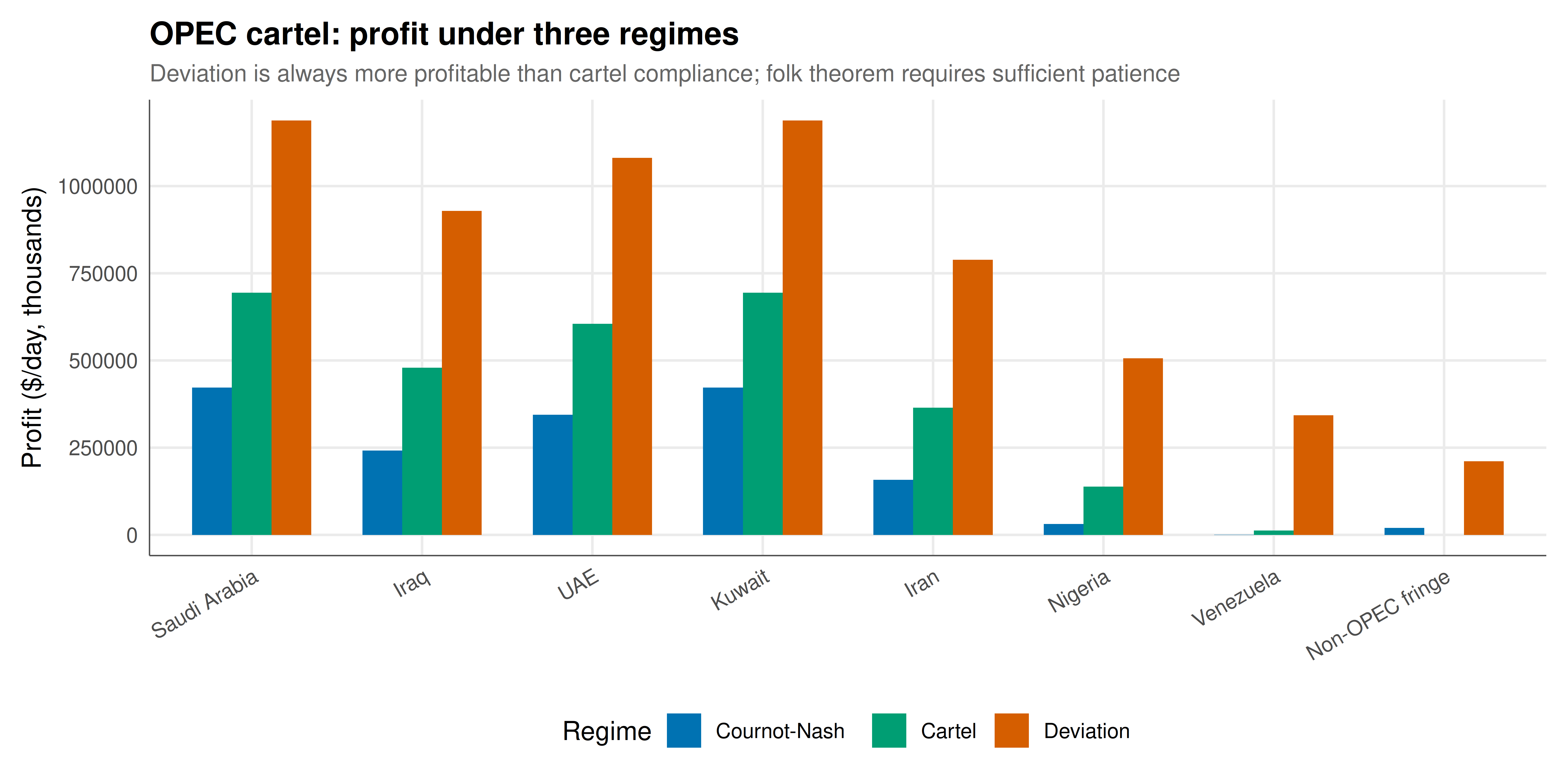
#| fig-cap: "Figure 1. Profit comparison across three regimes for each OPEC-style producer: Cournot-Nash (competitive), cartel (coordinated output restriction), and unilateral deviation from the cartel. Low-cost producers like Saudi Arabia gain the most from deviation, making them the most critical for cartel stability. Okabe-Ito palette."
#| dev: [png, pdf]
#| fig-width: 10
#| fig-height: 5
#| dpi: 300
profit_compare <- deviation_df |>
  select(Producer, Pi_Nash, Pi_Cartel, Pi_Deviate) |>
  pivot_longer(-Producer, names_to = "Regime", values_to = "Profit") |>
  mutate(
    Regime = factor(Regime,
      levels = c("Pi_Nash", "Pi_Cartel", "Pi_Deviate"),
      labels = c("Cournot-Nash", "Cartel", "Deviation")),
    Producer = factor(Producer, levels = producers$name)
  )

p_profits <- ggplot(profit_compare,
       aes(x = Producer, y = Profit, fill = Regime)) +
  geom_col(position = "dodge", width = 0.7) +
  scale_fill_manual(values = c("Cournot-Nash" = okabe_ito[5],
                                "Cartel" = okabe_ito[3],
                                "Deviation" = okabe_ito[6])) +
  labs(
    title = "OPEC cartel: profit under three regimes",
    subtitle = "Deviation is always more profitable than cartel compliance; folk theorem requires sufficient patience",
    x = NULL, y = "Profit ($/day, thousands)",
    fill = "Regime"
  ) +
  theme_publication() +
  theme(axis.text.x = element_text(angle = 30, hjust = 1))

p_profits
```
## Interactive figure
```{r}
#| label: fig-folk-theorem-interactive
folk_plot <- folk_df |>
  mutate(
    text = sprintf("Producers: %d\nCritical delta: %.4f\nSustainable at delta=0.9: %s",
                   n, delta_star,
                   ifelse(delta_star <= 0.9, "Yes", "No"))
  )

# Add deviation analysis data for hovertext
dev_plot <- deviation_df |>
  mutate(
    text = sprintf("%s (c = $%d)\nDelta*: %.4f\nCartel profit: $%s\nDeviation profit: $%s\nNash profit: $%s",
                   Producer, Cost, Delta_star,
                   format(Pi_Cartel, big.mark = ","),
                   format(Pi_Deviate, big.mark = ","),
                   format(Pi_Nash, big.mark = ","))
  )

p_folk <- ggplot(folk_plot, aes(x = n, y = delta_star, text = text)) +
  geom_line(color = okabe_ito[5], linewidth = 0.9) +
  geom_point(color = okabe_ito[5], size = 2) +
  geom_hline(yintercept = 0.9, linetype = "dashed", color = okabe_ito[6],
             linewidth = 0.5) +
  geom_hline(yintercept = 0.95, linetype = "dashed", color = okabe_ito[1],
             linewidth = 0.5) +
  annotate("text", x = 18, y = 0.88, label = "delta = 0.9",
           color = okabe_ito[6], size = 3.5) +
  annotate("text", x = 18, y = 0.93, label = "delta = 0.95",
           color = okabe_ito[1], size = 3.5) +
  scale_x_continuous(breaks = seq(2, 20, by = 2)) +
  labs(
    title = "Folk theorem: critical discount factor for cartel sustainability",
    subtitle = "Symmetric Cournot with linear demand; cartel harder to sustain as n increases",
    x = "Number of producers (n)",
    y = expression(paste("Critical discount factor ", delta, "*"))
  ) +
  theme_publication()

ggplotly(p_folk, tooltip = "text") |>
  config(displaylogo = FALSE,
         modeBarButtonsToRemove = c("select2d", "lasso2d"))
```
## Interpretation
The analysis reveals the fundamental tension at the heart of OPEC and any production cartel: the cartel creates substantial joint surplus relative to the competitive outcome, but each member has a powerful unilateral incentive to cheat. In our stylised model, the cartel increases total industry profits by restricting output to approximately two-thirds of the competitive level, raising the oil price significantly. Every member benefits from the higher price — even the highest-cost producer (Non-OPEC fringe at $35/barrel) earns more under the cartel than under competition. But the deviation column tells the critical story: each member can earn even more by secretly increasing production while others maintain their quotas. The deviating firm captures a larger share of the market at a price that, while lower than the cartel price, is still far above the competitive level (because only one firm has increased output). This one-period gain from cheating is the temptation that must be overcome for the cartel to survive.
The critical discount factor $\delta^*$ quantifies exactly how patient each member must be to resist this temptation. Under the grim trigger strategy — where any detected deviation triggers permanent reversion to the competitive Nash equilibrium — the cartel is sustainable only if every member's discount factor exceeds the maximum $\delta^*$ across all members. Our heterogeneous-cost model reveals an important asymmetry: the critical discount factor varies across producers. The producers with the most to gain from deviation relative to cartel compliance are those who face the most binding constraint. In our calibration, the low-cost producers (Saudi Arabia, Kuwait) have the largest deviation incentives because they can profitably flood the market at prices that would drive high-cost producers out. This is consistent with the historical record: Saudi Arabia's 1985 decision to increase production and abandon the swing producer role precipitated the 1986 oil price crash.
The folk theorem analysis with symmetric producers provides the broader structural insight: cartel stability deteriorates monotonically as the number of producers increases. With 2 producers, the critical discount factor is relatively modest — bilateral collusion is comparatively easy to sustain. As the number grows, each firm's share of the cartel profit shrinks (it is divided among more members), but the deviation gain remains large (the deviator captures a disproportionate share). With 13 producers (roughly OPEC's current membership), the critical discount factor is high, indicating that sustaining the cartel requires considerable patience and willingness to sacrifice short-term gains. The addition of OPEC+ partners (Russia, Kazakhstan, and others) further increases the effective $n$ and makes coordination even harder, which helps explain why OPEC+ agreements have been fragile and frequently tested by quota violations.
The model also illuminates why OPEC has adopted various institutional mechanisms to mitigate the cheating problem. Regular monitoring of production levels through satellite imagery and independent auditors serves as a detection mechanism — cheating is less attractive if it is quickly discovered. Saudi Arabia's historical role as swing producer functioned as a selective punishment mechanism: rather than triggering Nash reversion by all members, Saudi Arabia could selectively increase its own output to punish specific violators, a strategy that is cheaper (in terms of lost cartel rents) than full competitive reversion. The model could be extended to incorporate these richer strategy spaces, moving beyond simple grim trigger to optimal punishment schemes as characterised by Abreu (1986), which can sustain cooperation at lower discount factors.
Several features of real oil markets that our model abstracts from would further enrich the analysis. Demand uncertainty and supply shocks make it difficult to distinguish genuine cheating from random fluctuations — this is Green and Porter's (1984) classic insight about imperfect monitoring in cartels. Capacity constraints mean that producers cannot deviate arbitrarily far from their quotas. The exhaustibility of oil reserves introduces a dynamic dimension: producers must consider not only current-period profits but also the path of extraction over time, linking cartel theory to Hotelling's rule of resource economics. Entry by non-OPEC producers (particularly US shale) effectively increases $n$ endogenously in response to high cartel prices, a force that fundamentally undermines cartel sustainability in the long run. Despite these complexities, the basic Cournot framework captures the essential economics of OPEC's strategic problem: the perennial struggle between collective discipline and individual temptation.
## Extensions & related tutorials
- [Tragedy of the commons](../tragedy-of-the-commons/) — the public goods problem underlying common pool resource extraction, of which oil cartels are a special case.
- [Climate coalition formation](../climate-coalition-formation/) — modelling international environmental agreements as coalition formation games, with parallels to OPEC.
- [Spectrum auction design](../spectrum-auction-design/) — mechanism design for allocating scarce resources, contrasted with the cartel approach to restricting supply.
- [Voting power indices](../../cooperative-gt/voting-power-indices/) — measuring the influence of heterogeneous OPEC members in collective production decisions.
- [Shapley value and fair division](../../cooperative-gt/shapley-value/) — allocating cartel surplus fairly among heterogeneous members.
## References
::: {#refs}
:::