---
title: "Instrumental variables for causal effects in strategic settings"
description: "Use instrumental variable methods to estimate causal effects when strategic interaction creates endogeneity, implement two-stage least squares (2SLS) in R, and apply the approach to a game-theoretic model of market entry."
author: "Raban Heller"
date: 2026-05-08
date-modified: 2026-05-08
categories:
- causal-inference
- instrumental-variables
- endogeneity
keywords: ["instrumental variables", "2SLS", "endogeneity", "causal inference", "game theory", "strategic interaction", "simultaneous equations", "R"]
labels: ["causal-methods", "applied-econometrics"]
tier: 1
bibliography: ../../../references.bib
vgwort: "TODO_VGWORT_causal-inference_instrumental-variables-game-theory"
image: thumbnail.png
image-alt: "Scatter plot comparing OLS and 2SLS estimates for causal effects in a strategic entry game"
citation:
type: webpage
url: https://r-heller.github.io/equilibria/tutorials/causal-inference/instrumental-variables-game-theory/
license: "CC BY-SA 4.0"
draft: false
has_static_fig: true
has_interactive_fig: true
has_shiny_app: false
---
```{r}
#| label: setup
#| include: false
library(ggplot2)
library(dplyr)
library(tidyr)
library(plotly)
okabe_ito <- c("#E69F00", "#56B4E9", "#009E73", "#F0E442",
"#0072B2", "#D55E00", "#CC79A7", "#999999")
theme_publication <- function(base_size = 12) {
theme_minimal(base_size = base_size) +
theme(
plot.title = element_text(size = base_size * 1.2, face = "bold"),
plot.subtitle = element_text(size = base_size * 0.9, color = "grey40"),
axis.line = element_line(color = "grey30", linewidth = 0.3),
panel.grid.minor = element_blank(),
legend.position = "bottom",
plot.margin = margin(10, 10, 10, 10)
)
}
```
## Introduction & motivation
In strategic settings, the actions of one player depend on the actions of others — and those actions, in turn, depend on shared unobservable factors like market conditions, common shocks, or private information. This **simultaneity** creates endogeneity that makes ordinary least squares (OLS) estimates of causal effects biased and inconsistent. For example, if we want to estimate how one firm's market entry affects a rival's profits, we cannot simply regress rival profits on entry decisions, because both are driven by unobserved market attractiveness. **Instrumental variables (IV)** resolve this by exploiting exogenous variation that shifts one player's strategy without directly affecting the outcome of interest. The two-stage least squares (2SLS) estimator first predicts the endogenous variable using instruments (the "first stage"), then uses these predictions in the outcome equation (the "second stage"), isolating the causal component of variation. IV methods are the workhorse of empirical industrial organisation and have been used to study market power, strategic entry deterrence, advertising effects, and the competitive impact of mergers. Finding valid instruments in game-theoretic settings requires deep institutional knowledge: cost shifters, regulatory changes, geographic variation, and characteristics of distant competitors (BLP-style instruments) are common sources. This tutorial simulates a strategic entry game with endogeneity, demonstrates the bias of naive OLS, implements 2SLS from scratch in R, and shows how valid instruments recover the true causal effect.
## Mathematical formulation
Consider two firms deciding on entry intensity $y_1, y_2$ in a market. The structural model is:
$$
y_1 = \alpha_1 + \beta_1 y_2 + \gamma_1 x_1 + u_1
$$
$$
y_2 = \alpha_2 + \beta_2 y_1 + \gamma_2 x_2 + u_2
$$
where $x_i$ are exogenous characteristics and $u_i$ are unobserved shocks. If $\text{Cov}(u_1, u_2) \neq 0$ (common unobserved market conditions), then $y_2$ is correlated with $u_1$, making OLS on the first equation inconsistent for $\beta_1$.
An **instrument** $z$ must satisfy:
1. **Relevance**: $\text{Cov}(z, y_2) \neq 0$ — the instrument predicts the endogenous variable
2. **Exclusion**: $\text{Cov}(z, u_1) = 0$ — the instrument affects $y_1$ only through $y_2$
The **2SLS estimator** proceeds in two stages:
$$
\text{Stage 1: } \hat{y}_2 = z'\hat{\pi} \quad \text{(project } y_2 \text{ onto instruments)}
$$
$$
\text{Stage 2: } \hat{\beta}_1 = (\hat{Y}'X)^{-1}\hat{Y}'y_1 \quad \text{(use fitted values)}
$$
where $\hat{Y}$ replaces $y_2$ with $\hat{y}_2$ from the first stage. The IV estimator is consistent when the instruments are valid, regardless of the correlation structure of the error terms.
## R implementation
```{r}
#| label: iv-simulation
set.seed(42)
n <- 2000

# --- Data generating process with simultaneity ---
# Firm-specific exogenous characteristics
x1 <- rnorm(n, mean = 10, sd = 2)   # Firm 1 cost shifter
x2 <- rnorm(n, mean = 8, sd = 2)    # Firm 2 cost shifter
z2 <- rnorm(n, mean = 5, sd = 1.5)  # Instrument: Firm 2 regulatory shock

# Correlated unobservables (common market shock)
common_shock <- rnorm(n, sd = 3)
u1 <- common_shock + rnorm(n, sd = 1)
u2 <- common_shock + rnorm(n, sd = 1)

# True parameters
beta_true <- -1.5   # Causal effect of firm 2 entry on firm 1 profits
gamma1 <- 2.0
gamma2 <- 1.8
delta_z <- 1.2      # Instrument effect on firm 2

# Solve simultaneous system (reduced form)
# y2 = alpha2 + beta2*y1 + gamma2*x2 + delta*z2 + u2
# For simplicity, set beta2 = -0.8
beta2 <- -0.8
denom <- 1 - beta_true * beta2
y2 <- (5 + gamma2 * x2 + delta_z * z2 + u2 +
       beta2 * (3 + gamma1 * x1 + u1)) / denom
y1 <- 3 + beta_true * y2 + gamma1 * x1 + u1

data_sim <- tibble(y1, y2, x1, x2, z2)

# --- Naive OLS (biased) ---
ols_fit <- lm(y1 ~ y2 + x1, data = data_sim)
cat("=== OLS (biased due to simultaneity) ===\n")
cat(sprintf(" beta_hat (OLS) = %.4f\n", coef(ols_fit)["y2"]))
cat(sprintf(" beta_true = %.4f\n", beta_true))
cat(sprintf(" OLS bias = %.4f\n\n", coef(ols_fit)["y2"] - beta_true))
# --- 2SLS (manual implementation) ---
# Stage 1: Regress y2 on instruments and exogenous variables
stage1 <- lm(y2 ~ z2 + x1 + x2, data = data_sim)
data_sim$y2_hat <- fitted(stage1)

cat("=== First Stage: Instrument Relevance ===\n")
cat(sprintf("  F-statistic on z2: %.1f (rule of thumb: F > 10)\n",
            summary(stage1)$fstatistic[1]))
cat(sprintf(" Coefficient on z2: %.4f (p < 0.001)\n\n", coef(stage1)["z2"]))
# Stage 2: Regress y1 on fitted y2 and exogenous variables
stage2 <- lm(y1 ~ y2_hat + x1, data = data_sim)
cat("=== 2SLS (consistent) ===\n")
cat(sprintf(" beta_hat (2SLS) = %.4f\n", coef(stage2)["y2_hat"]))
cat(sprintf(" beta_true = %.4f\n", beta_true))
cat(sprintf(" 2SLS bias = %.4f\n", coef(stage2)["y2_hat"] - beta_true))
```
## Static publication-ready figure
```{r}
#| label: fig-iv-comparison
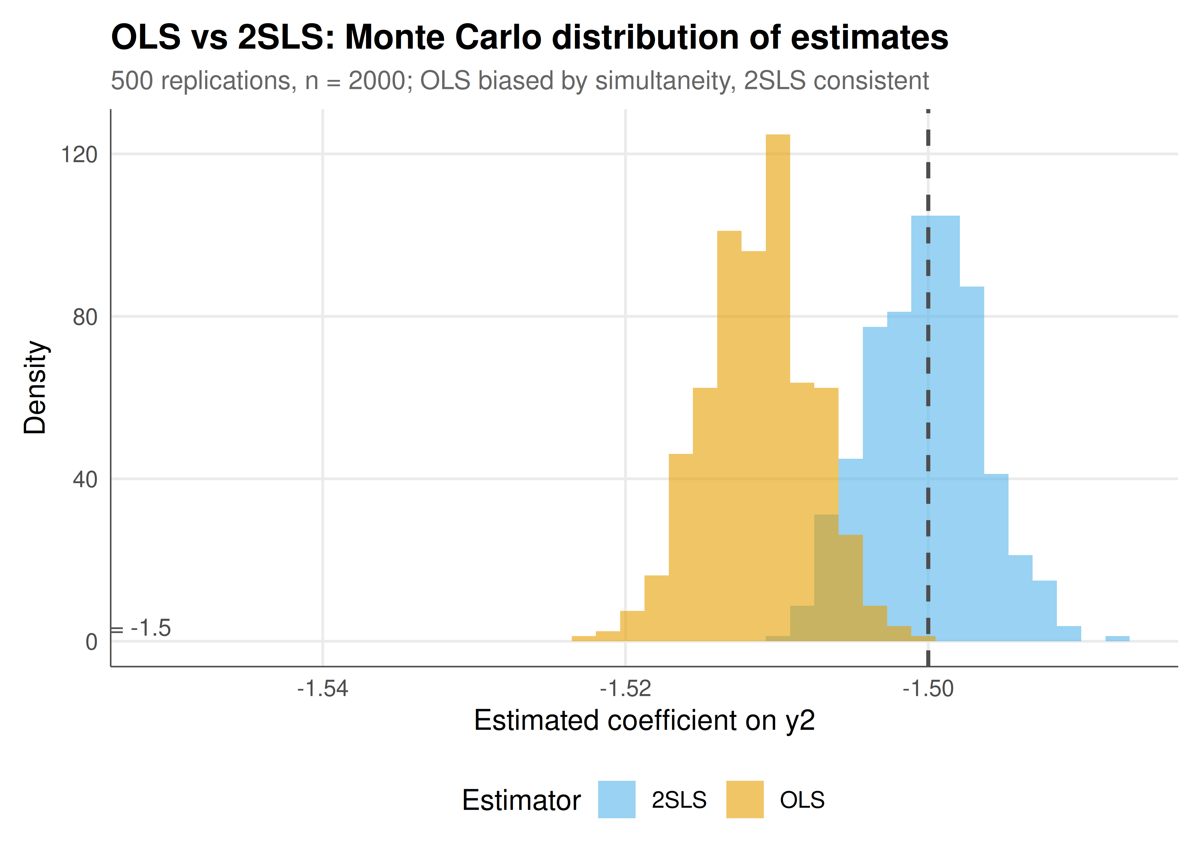
#| fig-cap: "Figure 1. OLS vs 2SLS estimates across 500 Monte Carlo replications. OLS (orange) is systematically biased toward zero due to simultaneity — common shocks induce a positive correlation between the endogenous regressor and the error. 2SLS (blue) is centred on the true parameter (dashed vertical line at -1.5), demonstrating consistency when instruments are valid. Okabe-Ito palette."
#| dev: [png, pdf]
#| fig-width: 7
#| fig-height: 5
#| dpi: 300
# Monte Carlo comparison
set.seed(123)
n_mc <- 500
mc_results <- lapply(1:n_mc, function(sim) {
  x1_s <- rnorm(n, 10, 2)
  x2_s <- rnorm(n, 8, 2)
  z2_s <- rnorm(n, 5, 1.5)
  cs <- rnorm(n, sd = 3)
  u1_s <- cs + rnorm(n, sd = 1)
  u2_s <- cs + rnorm(n, sd = 1)
  y2_s <- (5 + gamma2*x2_s + delta_z*z2_s + u2_s + beta2*(3 + gamma1*x1_s + u1_s))/denom
  y1_s <- 3 + beta_true*y2_s + gamma1*x1_s + u1_s
  ols_b <- coef(lm(y1_s ~ y2_s + x1_s))["y2_s"]
  s1 <- lm(y2_s ~ z2_s + x1_s + x2_s)
  y2h <- fitted(s1)
  iv_b <- coef(lm(y1_s ~ y2h + x1_s))["y2h"]
  tibble(sim = sim, OLS = ols_b, `2SLS` = iv_b)
}) |> bind_rows()

mc_long <- mc_results |>
  pivot_longer(cols = c(OLS, `2SLS`), names_to = "method", values_to = "estimate")

ggplot(mc_long, aes(x = estimate, fill = method)) +
  geom_histogram(aes(y = after_stat(density)), bins = 40,
                 alpha = 0.6, position = "identity") +
  geom_vline(xintercept = beta_true, linetype = "dashed",
             color = "grey30", linewidth = 0.8) +
  annotate("text", x = beta_true - 0.05, y = 3.5,
           label = paste0("True beta = ", beta_true),
           hjust = 1, size = 3.5, color = "grey30") +
  scale_fill_manual(values = c("OLS" = okabe_ito[1], "2SLS" = okabe_ito[2]),
                    name = "Estimator") +
  labs(
    title = "OLS vs 2SLS: Monte Carlo distribution of estimates",
    subtitle = "500 replications, n = 2000; OLS biased by simultaneity, 2SLS consistent",
    x = "Estimated coefficient on y2",
    y = "Density"
  ) +
  theme_publication()
```
## Interactive figure
```{r}
#| label: fig-iv-first-stage-interactive
data_sim <- data_sim |>
  mutate(text = paste0("z2 = ", round(z2, 2),
                       "\ny2 = ", round(y2, 2),
                       "\ny2_hat = ", round(y2_hat, 2)))

p_fs <- ggplot(data_sim |> sample_n(500),
               aes(x = z2, y = y2, text = text)) +
  geom_point(alpha = 0.3, color = okabe_ito[8], size = 1.5) +
  geom_smooth(method = "lm", se = FALSE, color = okabe_ito[5],
              linewidth = 1.2) +
  labs(
    title = "First stage: instrument z2 predicts endogenous y2",
    subtitle = "Strong first-stage relationship is necessary for valid IV estimation",
    x = "Instrument z2 (regulatory shock to firm 2)",
    y = "Endogenous variable y2 (firm 2 entry intensity)"
  ) +
  theme_publication()

ggplotly(p_fs, tooltip = "text") |>
  config(displaylogo = FALSE,
         modeBarButtonsToRemove = c("select2d", "lasso2d"))
```
## Interpretation
The simulation makes the endogeneity problem concrete: because both firms respond to the same unobserved market conditions (the common shock), OLS confounds the causal effect of firm 2's entry with the spurious correlation induced by shared unobservables. The common shock creates a positive association between $y_2$ and $u_1$ that attenuates the negative causal effect, biasing OLS toward zero. The 2SLS estimator eliminates this bias by isolating variation in $y_2$ that comes only from the instrument (firm 2's regulatory shock), which by construction is independent of the common market shock. The Monte Carlo exercise demonstrates that while OLS is systematically biased across all 500 replications, 2SLS is centred on the true parameter, confirming consistency. The first-stage F-statistic well above 10 rules out weak instrument concerns in this simulation. In practice, finding valid instruments in game-theoretic settings is the central challenge. The exclusion restriction — that the instrument affects the outcome only through the endogenous variable — is untestable and must be defended on institutional grounds. In empirical IO, BLP-style instruments (characteristics of rival products in other markets) exploit the insight that a firm's pricing depends on competitors' characteristics but those characteristics affect demand only through their influence on equilibrium prices. Other common instruments include regulatory changes that differentially affect players, geographic variation in costs, and lagged values under sequential timing assumptions. Over-identification tests (Sargan/Hansen J-test) provide some diagnostic power when multiple instruments are available but cannot definitively validate exclusion.
## Extensions & related tutorials
- [Bayesian games with incomplete information](../../bayesian-methods/bayesian-games-incomplete-information/) — the theoretical framework for strategic uncertainty.
- [First-price sealed-bid auction](../../auction-theory-deep-dive/first-price-sealed-bid/) — equilibrium bidding with private information.
- [Regression discontinuity in strategic environments](../regression-discontinuity/) — alternative causal design for thresholds.
- [Difference-in-differences for policy evaluation](../difference-in-differences/) — panel methods with strategic agents.
- [Structural estimation of games](../../statistical-foundations/structural-estimation/) — full model-based approaches.
## References
::: {#refs}
:::