---
title: "The Prisoner's Dilemma — formal setup and dominant strategy analysis"
description: "Define the one-shot Prisoner's Dilemma formally, prove that mutual defection is the unique dominant-strategy equilibrium, and explore how payoff parameters affect the tension between individual and collective rationality."
author: "Raban Heller"
date: 2026-05-08
date-modified: 2026-05-08
categories:
- classical-games
- prisoners-dilemma
- dominant-strategy
- social-dilemma
keywords: ["Prisoner's Dilemma", "dominant strategy", "social dilemma", "cooperation", "defection", "Pareto efficiency"]
labels: ["canonical-games", "social-dilemmas"]
tier: 1
bibliography: ../../../references.bib
vgwort: "TODO_VGWORT_classical-games_prisoners-dilemma-formal"
image: thumbnail.png
image-alt: "Payoff matrix of the Prisoner's Dilemma highlighting the dominant strategy equilibrium"
citation:
type: webpage
url: https://r-heller.github.io/equilibria/tutorials/classical-games/prisoners-dilemma-formal/
license: "CC BY-SA 4.0"
draft: false
has_static_fig: true
has_interactive_fig: true
has_shiny_app: false
---
```{r}
#| label: setup
#| include: false
library(ggplot2)
library(dplyr)
library(tidyr)
library(plotly)
okabe_ito <- c("#E69F00", "#56B4E9", "#009E73", "#F0E442",
"#0072B2", "#D55E00", "#CC79A7", "#999999")
theme_publication <- function(base_size = 12) {
theme_minimal(base_size = base_size) +
theme(
plot.title = element_text(size = base_size * 1.2, face = "bold"),
plot.subtitle = element_text(size = base_size * 0.9, color = "grey40"),
axis.line = element_line(color = "grey30", linewidth = 0.3),
panel.grid.minor = element_blank(),
legend.position = "bottom",
plot.margin = margin(10, 10, 10, 10)
)
}
```
## Introduction & motivation
The Prisoner's Dilemma (PD) is the most famous game in all of game theory — and arguably in all of social science. First formalised by Merrill Flood and Melvin Dresher at RAND in 1950 and given its narrative framing by Albert Tucker, the PD captures the fundamental tension between individual rationality and collective welfare: two players each have a dominant strategy to defect, yet mutual defection leaves both worse off than mutual cooperation. This paradox — that individually rational behaviour leads to a collectively irrational outcome — underpins problems ranging from arms races and climate change to price competition and the tragedy of the commons. The PD is not merely an academic exercise; it is the formal skeleton of any situation where short-term self-interest conflicts with long-term mutual benefit. Understanding the one-shot PD rigorously — its payoff constraints, the proof that defection is dominant, the Pareto inefficiency of the equilibrium, and how parameter changes affect the severity of the dilemma — is prerequisite for every extension: the iterated PD, spatial PD, stochastic PD, and the vast literature on mechanisms that can sustain cooperation.
## Mathematical formulation
The **Prisoner's Dilemma** is a symmetric two-player game with strategy set $\{C, D\}$ (Cooperate, Defect) and payoff matrix:
$$
\begin{array}{c|cc}
& C & D \\ \hline
C & R, R & S, T \\
D & T, S & P, P
\end{array}
$$
subject to two constraints:
1. **Temptation ordering**: $T > R > P > S$ — defecting against a cooperator is the best outcome; mutual defection beats being exploited.
2. **Efficiency constraint**: $2R > T + S$ — mutual cooperation is more efficient than alternating exploitation.
**Proposition**: Defect is a strictly dominant strategy for both players, and $(D, D)$ is the unique Nash equilibrium.
*Proof*: For the row player, regardless of the column player's action: $T > R$ (prefer D when opponent plays C) and $P > S$ (prefer D when opponent plays D). Since $D$ strictly dominates $C$, rational players always defect. $\square$
The equilibrium payoff $P$ is Pareto-dominated by $R$ — both players would prefer $(C, C)$, but no unilateral deviation from $(D, D)$ can achieve it.
## R implementation
```{r}
#| label: pd-analysis
# Parameterized PD analysis
pd_analysis <- function(T_val, R_val, P_val, S_val) {
  # Verify PD constraints
  stopifnot(T_val > R_val, R_val > P_val, P_val > S_val)
  stopifnot(2 * R_val > T_val + S_val)

  # Dilemma strength metrics
  temptation_gain <- T_val - R_val     # gain from unilateral defection
  sucker_cost <- P_val - S_val         # cost avoided by defecting when opponent defects
  cooperation_premium <- R_val - P_val  # value of mutual cooperation over mutual defection
  efficiency_gap <- 2 * R_val - (T_val + S_val)  # margin on efficiency constraint

  list(
    payoff_matrix = matrix(c(R_val, S_val, T_val, P_val), nrow = 2,
                            dimnames = list(c("C","D"), c("C","D"))),
    temptation_gain = temptation_gain,
    sucker_cost = sucker_cost,
    cooperation_premium = cooperation_premium,
    efficiency_gap = efficiency_gap,
    dilemma_strength = temptation_gain / cooperation_premium
  )
}

# Axelrod's standard parameterization
cat("=== Axelrod parameterization (T=5, R=3, P=1, S=0) ===\n")
ax <- pd_analysis(5, 3, 1, 0)
cat("Payoff matrix:\n"); print(ax$payoff_matrix)
cat(sprintf("Temptation gain: %d\nSucker cost: %d\nCooperation premium: %d\n",
            ax$temptation_gain, ax$sucker_cost, ax$cooperation_premium))
cat(sprintf("Dilemma strength (temptation/premium): %.2f\n\n", ax$dilemma_strength))
# Weak dilemma
cat("=== Weak dilemma (T=4, R=3, P=1, S=0) ===\n")
weak <- pd_analysis(4, 3, 1, 0)
cat(sprintf("Dilemma strength: %.2f\n\n", weak$dilemma_strength))
# Strong dilemma
cat("=== Strong dilemma (T=10, R=3, P=1, S=-5) ===\n")
strong <- pd_analysis(10, 3, 1, -5)
cat(sprintf("Dilemma strength: %.2f\n", strong$dilemma_strength))
```
## Static publication-ready figure
```{r}
#| label: fig-pd-payoff-space
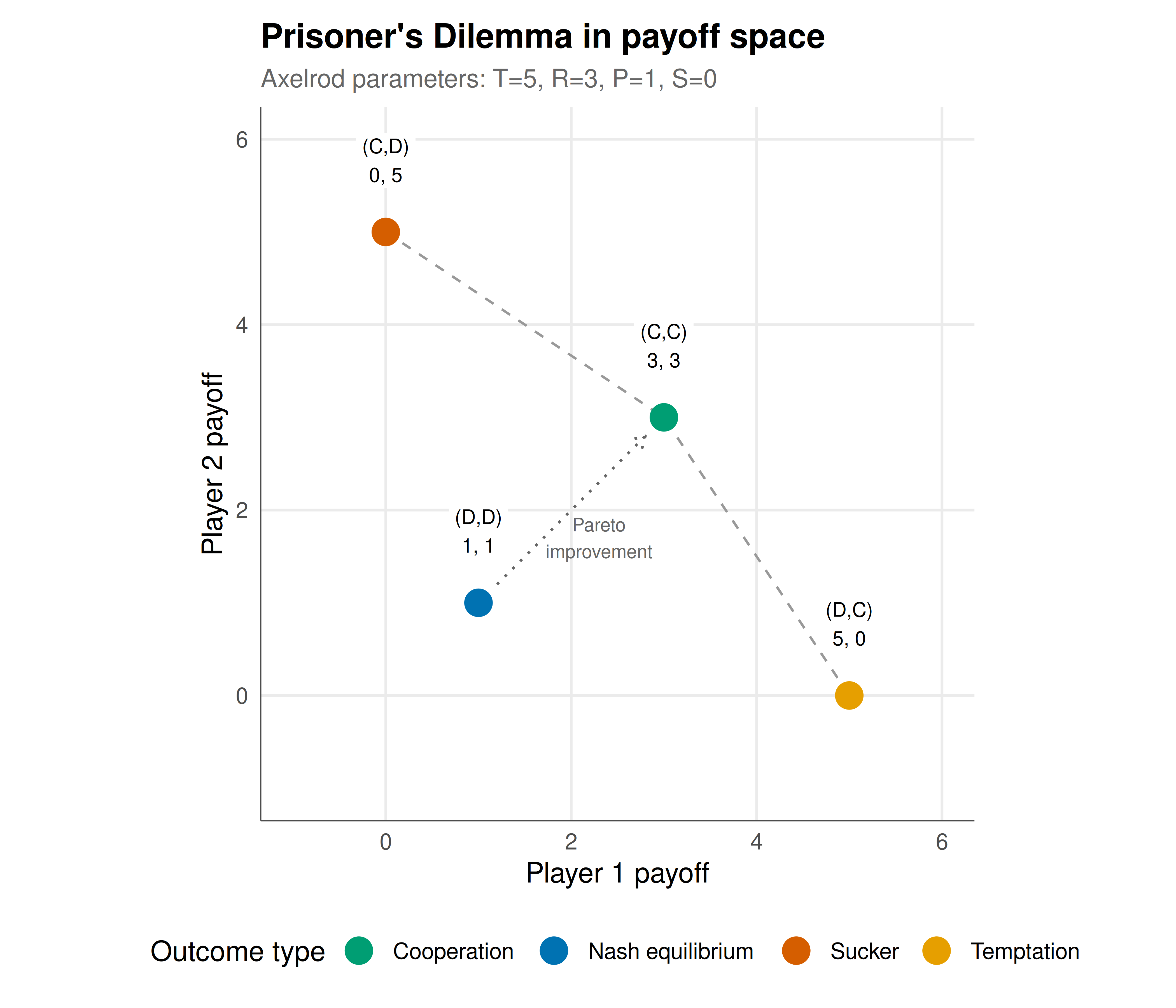
#| fig-cap: "Figure 1. The four outcomes of the Prisoner's Dilemma in payoff space. Mutual cooperation (R, R) Pareto-dominates the Nash equilibrium (P, P), but each player is individually tempted to defect to (T, S). The dashed line marks Pareto efficiency; the PD equilibrium lies strictly below it — the hallmark of a social dilemma. Okabe-Ito palette."
#| dev: [png, pdf]
#| fig-width: 7
#| fig-height: 6
#| dpi: 300
# Payoff space for Axelrod's PD
outcomes <- tibble(
  label = c("(C,C)", "(C,D)", "(D,C)", "(D,D)"),
  u1 = c(3, 0, 5, 1),
  u2 = c(3, 5, 0, 1),
  type = c("Cooperation", "Sucker", "Temptation", "Nash equilibrium")
)

# Pareto frontier: convex hull of Pareto-efficient outcomes
pareto_line <- tibble(u1 = c(0, 3, 5), u2 = c(5, 3, 0))

p_pd <- ggplot(outcomes, aes(x = u1, y = u2)) +
  # Pareto frontier
  geom_line(data = pareto_line, aes(x = u1, y = u2),
            linetype = "dashed", color = "grey60", linewidth = 0.5) +
  # Arrow from NE to cooperation
  annotate("segment", x = 1.2, y = 1.2, xend = 2.8, yend = 2.8,
           arrow = arrow(length = unit(0.2, "cm")), color = "grey40",
           linetype = "dotted") +
  annotate("text", x = 2.3, y = 1.7, label = "Pareto\nimprovement",
           size = 2.8, color = "grey40") +
  # Outcome points
  geom_point(aes(color = type), size = 5) +
  geom_label(aes(label = paste0(label, "\n", u1, ", ", u2)),
             vjust = -0.8, size = 3, fill = "white", label.size = 0) +
  scale_color_manual(values = c("Cooperation" = okabe_ito[3],
                                  "Sucker" = okabe_ito[6],
                                  "Temptation" = okabe_ito[1],
                                  "Nash equilibrium" = okabe_ito[5]),
                      name = "Outcome type") +
  coord_fixed(xlim = c(-1, 6), ylim = c(-1, 6)) +
  labs(
    title = "Prisoner's Dilemma in payoff space",
    subtitle = "Axelrod parameters: T=5, R=3, P=1, S=0",
    x = "Player 1 payoff", y = "Player 2 payoff"
  ) +
  theme_publication()

p_pd
```
## Interactive figure
```{r}
#| label: fig-pd-parameter-space
# Explore how dilemma strength varies across valid PD parameterizations
# Fix R=3, P=1, vary T and S within PD constraints
param_grid <- expand.grid(
  T_val = seq(3.1, 8, by = 0.1),
  S_val = seq(-3, 0.9, by = 0.1)
) |>
  filter(2 * 3 > T_val + S_val) |>  # efficiency constraint
  mutate(
    R = 3, P = 1,
    temptation_gain = T_val - R,
    cooperation_premium = R - P,
    dilemma_strength = temptation_gain / cooperation_premium,
    text = paste0("T=", round(T_val,1), ", S=", round(S_val,1),
                  "\nDilemma strength: ", round(dilemma_strength, 2))
  )

p_param <- ggplot(param_grid, aes(x = T_val, y = S_val, fill = dilemma_strength, text = text)) +
  geom_tile() +
  scale_fill_gradient2(low = okabe_ito[3], mid = okabe_ito[4], high = okabe_ito[6],
                        midpoint = 2, name = "Dilemma\nstrength") +
  geom_point(aes(x = 5, y = 0), shape = 4, size = 3, stroke = 2, color = "black") +
  annotate("text", x = 5.3, y = 0.3, label = "Axelrod", size = 3) +
  labs(
    title = "Prisoner's Dilemma parameter space",
    subtitle = "Dilemma strength = (T−R)/(R−P) with R=3, P=1; stronger = harder to sustain cooperation",
    x = "Temptation payoff (T)", y = "Sucker payoff (S)"
  ) +
  theme_publication() +
  theme(panel.grid = element_blank())

ggplotly(p_param, tooltip = "text") |>
  config(displaylogo = FALSE,
         modeBarButtonsToRemove = c("select2d", "lasso2d"))
```
## Interpretation
The Prisoner's Dilemma's power lies in its generality: any situation satisfying $T > R > P > S$ and $2R > T + S$ has the same qualitative structure — individual rationality leads to collective suboptimality. The dilemma strength metric reveals that the severity of this tension varies continuously: when the temptation gain is small relative to the cooperation premium (weak dilemma), the cost of defection is modest and cooperation may be easier to sustain through repeated interaction or social norms. When the dilemma is strong — high temptation, severe sucker payoff — sustaining cooperation requires more robust mechanisms: binding contracts, third-party enforcement, reputation systems, or sufficiently long time horizons in repeated play. The payoff-space visualization shows the geometric nature of the dilemma: the Nash equilibrium sits inside the Pareto frontier, with a Pareto improvement available but individually unattainable. The parameter space exploration reveals that the PD constraint region is bounded by the efficiency condition $2R > T + S$ — without this constraint, the game would not be a true dilemma because alternating exploitation could be efficient. Every extension in the #equilibria collection — iterated PD, spatial PD, evolutionary dynamics, mechanism design — is fundamentally about escaping this trap through some structural modification of the one-shot game analysed here.
## Extensions & related tutorials
- [The iterated PD — Axelrod's tournaments](../iterated-prisoners-dilemma-axelrod/) — cooperation through repetition.
- [Spatial PD on a lattice](../../simulations/spatial-prisoners-dilemma-nowak-may/) — cooperation through spatial structure.
- [Dominant strategies and IESDS](../../foundations/dominant-strategies-iterated-elimination/) — the general dominance framework.
- [Stag Hunt — coordination vs. risk](../stag-hunt/) — a related social dilemma with different equilibrium structure.
- [Folk theorem for repeated games](../../foundations/folk-theorem/) — theoretical foundations for escaping the PD trap.
## References
::: {#refs}
:::