Analyse the sealed-bid war of attrition as an all-pay second-price auction, derive the symmetric Bayesian Nash equilibrium with exponential bidding strategies for uniform private values, and compare revenue and surplus with the standard all-pay auction.
Author
Raban Heller
Published
May 8, 2026
Modified
May 8, 2026
Keywords
war of attrition, sealed-bid, all-pay auction, second-price, Bayesian Nash equilibrium, revenue equivalence, bidder surplus, R
Introduction & motivation
The war of attrition is one of the most fascinating and counterintuitive games in economic theory. Originally introduced by Maynard Smith in 1974 in the context of evolutionary biology to model animal conflicts where two contestants compete for a resource by persisting until one gives up, the war of attrition has since found applications across economics, political science, and industrial organization. In its most common continuous-time formulation, two players simultaneously choose how long they are willing to wait or fight. Both players incur costs proportional to the time spent in the contest, and the player who persists longer wins the prize. The loser has wasted all the time and resources spent waiting. This structure creates a strategic tension: staying in the contest is costly, but dropping out means conceding the prize.
The sealed-bid version of the war of attrition translates this dynamic conflict into a static mechanism design framework. In the sealed-bid war of attrition, each player simultaneously submits a bid representing their willingness to persist. Both players pay the lower of the two bids (reflecting the cost both incur up to the moment one drops out), and the higher bidder wins the prize. This makes the sealed-bid war of attrition an all-pay auction with second-price payment: “all-pay” because the loser also pays, and “second-price” because the payment equals the losing bid rather than the winning bid.
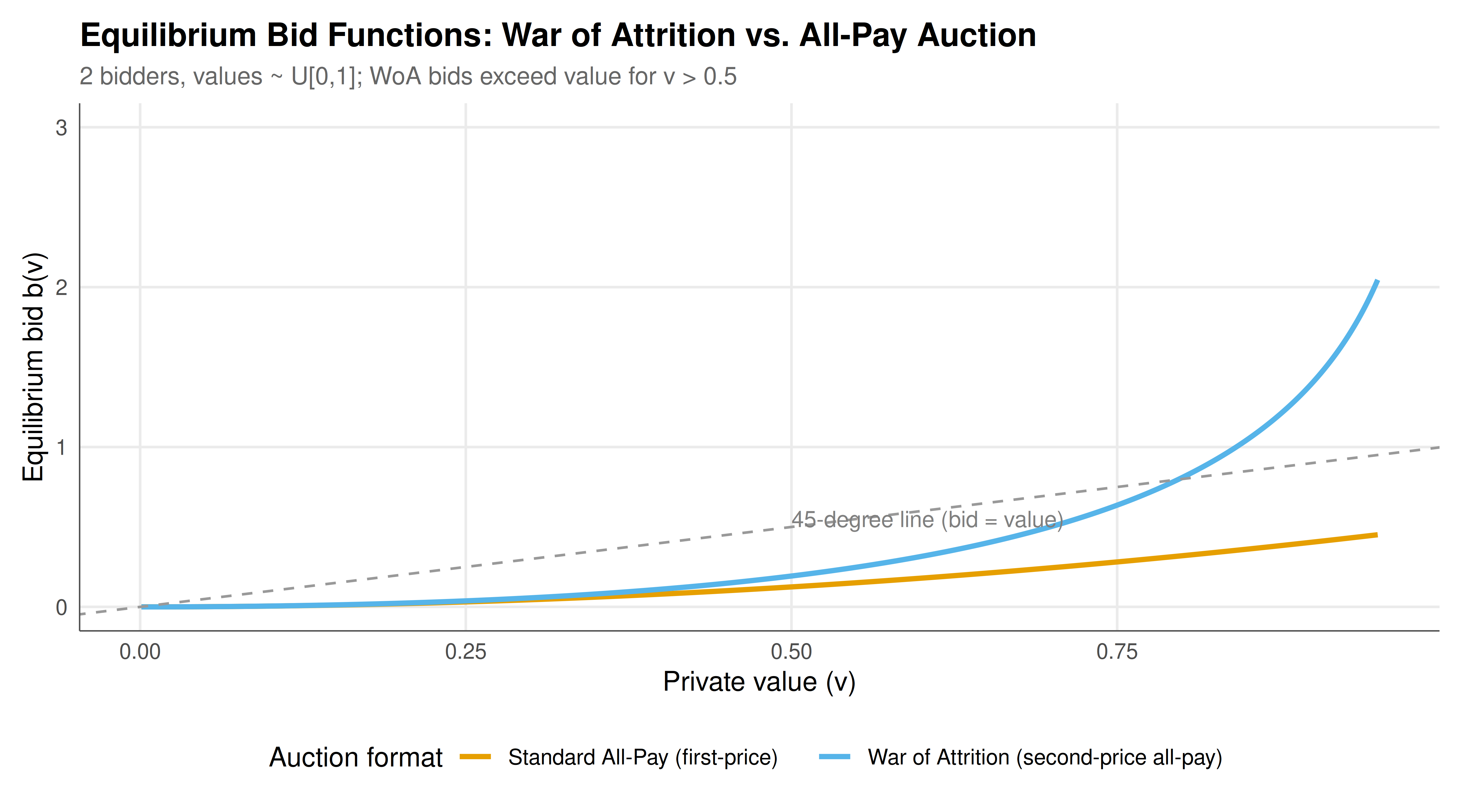
This payment rule creates dramatically different incentive structures compared to the standard (first-price) all-pay auction. In a first-price all-pay auction, each bidder pays their own bid regardless of winning or losing. The equilibrium bidding strategy in the first-price all-pay auction with two bidders and uniform values on [0, 1] is \(b(v) = v^2/2\), which is concave – high-value bidders bid conservatively because they already have a good chance of winning. In the sealed-bid war of attrition, the second-price payment rule changes the calculation fundamentally. Because a bidder’s payment is determined by the opponent’s bid (not their own), there is less cost to bidding high. In equilibrium, bidders with high values bid very aggressively – so aggressively, in fact, that the equilibrium bid function grows exponentially and bids can exceed the prize value. This seemingly irrational overbidding is rational because the expected payment (which depends on the opponent’s bid) is much lower than the bid itself.
The war of attrition structure appears in many real-world settings. Patent races, where firms invest in R&D hoping to be the first to develop a new technology, have a war-of-attrition flavour: all firms bear the cost of R&D, but only the winner profits from the patent. Price wars between firms competing for market share involve mutual losses until one firm exits. Political standoffs, such as government shutdowns or trade disputes, can persist well past the point where both sides have incurred substantial costs, because neither is willing to concede. In all these settings, the key feature is that both sides pay costs that depend on the shorter duration (or lower bid), and only the more persistent player captures the surplus.
The revenue equivalence theorem tells us that under certain conditions (independent private values, symmetric bidders, the same allocation rule), all auction formats generate the same expected revenue to the seller. The sealed-bid war of attrition and the standard all-pay auction both allocate the object to the highest bidder and require both bidders to pay, so they satisfy the conditions for revenue equivalence. Despite their very different bid functions and risk profiles, they generate identical expected revenue. However, the distribution of revenue can differ: the war of attrition tends to have higher variance in revenue because of the explosive bid function.
In this tutorial, we derive the symmetric Bayesian Nash equilibrium for the sealed-bid war of attrition with two bidders whose values are independently and uniformly distributed on [0, 1]. We implement the equilibrium bid function, simulate auctions to verify the theoretical predictions, compare revenue and surplus with the standard first-price all-pay auction, and analyse the distribution of outcomes for both formats. The analysis illustrates how the same allocation rule (highest bidder wins) can be implemented through radically different payment mechanisms with identical expected but very different realized outcomes.
Mathematical formulation
Consider two risk-neutral bidders with independent private values \(v_1, v_2 \sim U[0, 1]\). Each bidder submits a sealed bid \(b_i\). The higher bidder wins the prize of value \(v_i\) to bidder \(i\). Both bidders pay the minimum of the two bids.
Bidder \(i\)’s payoff given values \(v_i\) and bids \(b_i, b_j\):
Symmetric BNE derivation. Assume a symmetric, strictly increasing equilibrium bid function \(\beta(v)\). Bidder \(i\) with value \(v\) chooses bid \(b\) to maximize expected payoff:
\[
\max_b \; \Pr(\beta(v_j) < b) \cdot v - E[\beta(v_j) \mid \beta(v_j) < b]
\]
Since \(v_j \sim U[0,1]\) and \(\beta\) is increasing, \(\Pr(\beta(v_j) < b) = \beta^{-1}(b)\). Let \(z = \beta^{-1}(b)\). The expected payoff becomes:
\[
\Pi(z; v) = z \cdot v - \int_0^z \beta(s)\, ds
\]
Taking the first-order condition \(\partial \Pi / \partial z = 0\) and evaluating at the symmetric equilibrium where \(z = v\):
\[
v + v \cdot \beta'(v) - \beta(v) = 0 \quad \Longrightarrow \quad \beta'(v) - \frac{\beta(v)}{v} = -1
\]
Wait – let us redo this carefully. The expected payoff of bidding as if value is \(z\) (i.e., bidding \(\beta(z)\)) when true value is \(v\):
\[
\Pi(z; v) = z \cdot v - \int_0^z \beta(s)\, ds
\]
FOC: \(v = \beta(z)\), evaluated at \(z = v\) gives \(\beta(v) = v\). But this is the first-price all-pay auction solution. For the war of attrition, the payment is different.
Correcting: in the war of attrition, bidder \(i\)’s expected payment when bidding \(b = \beta(z)\) and opponent uses \(\beta\):
Actually, since both pay the lower bid: if \(i\) bids \(\beta(z)\) and wins (\(v_j < z\)), payment is \(\beta(v_j)\). If \(i\) loses (\(v_j > z\)), payment is \(\beta(z)\). So:
\[
\Pi(z; v) = z \cdot v - \int_0^z \beta(s)\,ds - (1 - z)\beta(z)
\]
For comparison, the first-price all-pay auction BNE is \(\beta^{\text{AP}}(v) = v^2 / 2\).
R implementation
We implement both bid functions, simulate 50,000 auctions under each format, and compare revenue, surplus, and outcome distributions.
set.seed(789)n_sim<-50000# --- Equilibrium bid functions ---beta_woa<-function(v)-v-log(1-v)# War of attrition (second-price all-pay)beta_ap<-function(v)v^2/2# Standard all-pay (first-price)# --- Simulate auctions ---v1<-runif(n_sim)v2<-runif(n_sim)# War of attritionb1_woa<-beta_woa(v1)b2_woa<-beta_woa(v2)winner_woa<-ifelse(b1_woa>b2_woa, 1, 2)payment_woa<-pmin(b1_woa, b2_woa)# both pay the lower bidrevenue_woa<-2*payment_woa# total payment by both bidders# Winner surplussurplus_winner_woa<-ifelse(winner_woa==1,v1-payment_woa,v2-payment_woa)# Loser surplus (negative)surplus_loser_woa<--payment_woa# Standard all-pay auctionb1_ap<-beta_ap(v1)b2_ap<-beta_ap(v2)winner_ap<-ifelse(b1_ap>b2_ap, 1, 2)revenue_ap<-b1_ap+b2_ap# each pays own bidsurplus_winner_ap<-ifelse(winner_ap==1,v1-b1_ap,v2-b2_ap)surplus_loser_ap<-ifelse(winner_ap==1, -b2_ap, -b1_ap)cat("=== Bid Function Comparison ===\n")
v = 0.1 0.0054 0.0050
v = 0.2 0.0231 0.0200
v = 0.3 0.0567 0.0450
v = 0.4 0.1108 0.0800
v = 0.5 0.1931 0.1250
v = 0.6 0.3163 0.1800
v = 0.7 0.5040 0.2450
v = 0.8 0.8094 0.3200
v = 0.9 1.4026 0.4050
cat(sprintf("WoA winner surplus: mean = %.4f\n", mean(surplus_winner_woa)))
WoA winner surplus: mean = 0.4989
cat(sprintf("WoA loser surplus: mean = %.4f\n", mean(surplus_loser_woa)))
WoA loser surplus: mean = -0.1685
cat(sprintf("AP winner surplus: mean = %.4f\n", mean(surplus_winner_ap)))
AP winner surplus: mean = 0.4170
cat(sprintf("AP loser surplus: mean = %.4f\n", mean(surplus_loser_ap)))
AP loser surplus: mean = -0.0841
cat(sprintf("\nWoA total expected surplus: %.4f\n",mean(surplus_winner_woa)+mean(surplus_loser_woa)))
WoA total expected surplus: 0.3304
cat(sprintf("AP total expected surplus: %.4f\n",mean(surplus_winner_ap)+mean(surplus_loser_ap)))
AP total expected surplus: 0.3330
# Efficiency check: does the highest-value bidder win?efficient_woa<-mean((winner_woa==1&v1>v2)|(winner_woa==2&v2>v1))efficient_ap<-mean((winner_ap==1&v1>v2)|(winner_ap==2&v2>v1))cat(sprintf("\nAllocative efficiency: WoA = %.4f, AP = %.4f\n",efficient_woa, efficient_ap))
Allocative efficiency: WoA = 1.0000, AP = 1.0000
Static publication-ready figure
The static figure shows the equilibrium bid functions for both auction formats side by side, highlighting the dramatic difference in bidding behaviour despite revenue equivalence.
v_grid<-seq(0.001, 0.95, length.out =500)bid_df<-data.frame( value =rep(v_grid, 2), bid =c(beta_woa(v_grid), beta_ap(v_grid)), format =rep(c("War of Attrition (second-price all-pay)","Standard All-Pay (first-price)"), each =length(v_grid)))p_bids<-ggplot(bid_df, aes(x =value, y =bid, color =format))+geom_line(linewidth =1.1)+geom_abline(slope =1, intercept =0, linetype ="dashed", color ="grey60")+scale_color_manual(values =okabe_ito[c(1, 2)])+annotate("text", x =0.5, y =0.55, label ="45-degree line (bid = value)", color ="grey50", size =3.5, hjust =0)+labs(title ="Equilibrium Bid Functions: War of Attrition vs. All-Pay Auction", subtitle ="2 bidders, values ~ U[0,1]; WoA bids exceed value for v > 0.5", x ="Private value (v)", y ="Equilibrium bid b(v)", color ="Auction format")+coord_cartesian(ylim =c(0, 3))+theme_publication()+theme(legend.position ="bottom")p_bids
Figure 1: Figure 1. Equilibrium bid functions for the sealed-bid war of attrition (exponential growth) and standard all-pay auction (quadratic). Despite radically different bid levels, both formats generate identical expected revenue of 1/3 under uniform values on [0,1]. The war of attrition’s explosive bid function reflects the second-price payment rule: bidders bid far above their values because they expect to pay only the losing bid. Data: analytical (CC BY-SA 4.0).
Interactive figure
The interactive version displays the revenue distribution for both formats, allowing the user to compare the spread and shape of revenue outcomes.
rev_df<-data.frame( revenue =c(revenue_woa, revenue_ap), format =rep(c("War of Attrition", "All-Pay Auction"), each =n_sim))# Sample for performanceset.seed(42)rev_sample<-rev_df|>group_by(format)|>slice_sample(n =5000)|>ungroup()rev_sample$text<-paste0("Format: ", rev_sample$format,"\nRevenue: $", round(rev_sample$revenue, 4))p_rev<-ggplot(rev_sample, aes(x =revenue, fill =format, text =text))+geom_histogram(aes(y =after_stat(density)), bins =60, alpha =0.6, position ="identity")+scale_fill_manual(values =okabe_ito[c(1, 2)])+geom_vline(xintercept =1/3, linetype ="dashed", color ="grey30")+annotate("text", x =1/3+0.02, y =2.5, label ="E[Revenue] = 1/3", size =3, hjust =0, color ="grey30")+labs(title ="Revenue Distribution: War of Attrition vs. All-Pay", x ="Total Revenue", y ="Density", fill ="Format")+coord_cartesian(xlim =c(0, 2))+theme_publication()ggplotly(p_rev, tooltip ="text")|>config(displaylogo =FALSE)