---
title: "Surveillance and privacy as a strategic equilibrium"
description: "A game-theoretic analysis of the surveillance-privacy tension modeled as an inspection game between a monitoring authority and citizens, with equilibrium computation, welfare analysis, and interactive visualizations of deterrence thresholds."
author: "Raban Heller"
date: 2026-05-08
date-modified: 2026-05-08
categories:
- ethics-applications
- inspection-games
- privacy
- surveillance
keywords: ["surveillance game", "inspection game", "privacy equilibrium", "deterrence", "monitoring intensity"]
labels: ["inspection-game", "privacy", "welfare-analysis", "mixed-strategy"]
tier: 1
bibliography: ../../../references.bib
vgwort: "TODO_VGWORT_ethics-applications_surveillance-privacy-equilibrium"
image: thumbnail.png
image-alt: "Line plot showing the equilibrium surveillance intensity and citizen compliance rate as functions of penalty severity, rendered using the Okabe-Ito palette."
citation:
type: webpage
url: https://r-heller.github.io/equilibria/tutorials/ethics-applications/surveillance-privacy-equilibrium/
license: "CC BY-SA 4.0"
draft: false
has_static_fig: true
has_interactive_fig: true
has_shiny_app: false
---
```{r}
#| label: setup
#| include: false
library(ggplot2)
library(dplyr)
library(tidyr)
library(plotly)
okabe_ito <- c("#E69F00", "#56B4E9", "#009E73", "#F0E442",
"#0072B2", "#D55E00", "#CC79A7", "#999999")
theme_publication <- function(base_size = 12) {
theme_minimal(base_size = base_size) +
theme(plot.title = element_text(size = base_size * 1.2, face = "bold"),
plot.subtitle = element_text(size = base_size * 0.9, color = "grey40"),
axis.line = element_line(color = "grey30", linewidth = 0.3),
panel.grid.minor = element_blank(), legend.position = "bottom",
plot.margin = margin(10, 10, 10, 10))
}
```
## Introduction and motivation
The tension between surveillance and privacy represents one of the most consequential strategic interactions in modern societies. Governments and corporations invest heavily in monitoring technologies -- from CCTV networks and internet traffic analysis to biometric identification systems -- while citizens simultaneously adopt privacy-enhancing technologies, modify their behavior, and advocate for legal protections against intrusive observation. This tension is not merely a policy debate but a genuine strategic interaction where each side's optimal behavior depends critically on the choices of the other.
Game theory, and specifically the theory of inspection games, provides a rigorous framework for analyzing this interaction. Inspection games were originally developed in the context of arms control verification during the Cold War, where inspectors needed to determine how frequently to verify treaty compliance given costly inspection procedures and the possibility that the inspected party might attempt to cheat. The same mathematical structure applies directly to surveillance: a monitoring authority must decide how intensively to surveil (the inspection probability), while citizens must decide whether to comply with regulations or engage in proscribed activities (the compliance decision).
The key insight from inspection game theory is that in equilibrium, both parties typically randomize. The monitoring authority cannot afford to inspect constantly (it is too costly), and the citizen cannot afford to always comply or always defect (the former sacrifices beneficial private activities, the latter risks detection and punishment). The resulting mixed-strategy equilibrium determines an optimal monitoring intensity and an equilibrium compliance rate, both of which depend on the underlying parameters: the cost of surveillance, the penalty for detected violations, the benefit of non-compliance to the citizen, and the authority's payoff from detecting violations versus the cost of false security.
This framework illuminates several important policy questions. First, it reveals the deterrence paradox: increasing penalties for detected violations actually reduces the equilibrium monitoring intensity rather than increasing it. When penalties are high, the authority needs to inspect less frequently to maintain the same deterrence effect. Second, welfare analysis shows that there can exist Pareto-improving reforms -- changes in the penalty-monitoring structure that make both sides better off. Third, the model highlights the importance of commitment: an authority that can credibly commit to a monitoring schedule (rather than choosing optimally in each period) may achieve higher welfare outcomes.
The relevance of this analysis has only grown with the expansion of digital surveillance capabilities. Modern surveillance technologies have dramatically reduced the cost of monitoring, shifting the equilibrium toward higher surveillance intensity and raising fundamental questions about the optimal balance between security and privacy. By formalizing this trade-off in game-theoretic terms, we can move beyond purely normative arguments and analyze the structural incentives that shape surveillance regimes.
In this tutorial, we construct a complete inspection game model, derive the mixed-strategy Nash equilibrium analytically, implement the solution in R, and visualize how equilibrium behavior and welfare respond to changes in key parameters. The analysis provides a foundation for understanding the strategic logic behind surveillance policy and its implications for individual privacy.
## Mathematical formulation
Consider a two-player game between an **Authority** (A) and a **Citizen** (C).
**Actions.** The Authority chooses monitoring intensity $m \in [0, 1]$. The Citizen chooses compliance probability $c \in [0, 1]$.
**Payoff parameters:**
- $b$: Citizen's benefit from non-compliance (violation payoff)
- $f$: Fine/penalty imposed on detected violators
- $k$: Authority's cost of monitoring per unit of intensity
- $d$: Authority's damage from undetected violations
**Citizen's expected payoff:**
$$
U_C(c, m) = c \cdot 0 + (1 - c)\bigl[b - m \cdot f\bigr] = (1 - c)(b - mf)
$$
**Authority's expected payoff:**
$$
U_A(m, c) = -(1 - c)(1 - m) \cdot d + (1 - c) \cdot m \cdot f - m \cdot k
$$
**Mixed-strategy Nash equilibrium.** The Citizen is indifferent when $b - m^* f = 0$:
$$
m^* = \frac{b}{f}
$$
The Authority is indifferent when the marginal benefit of monitoring equals its marginal cost:
$$
(1 - c^*)(d + f) = k \quad \Longrightarrow \quad c^* = 1 - \frac{k}{d + f}
$$
**Equilibrium welfare:**
$$
W^* = U_A^* + U_C^* = -\frac{k \cdot d}{d + f} - \frac{b \cdot k}{f}
$$
## R implementation
```{r}
#| label: surveillance-model
set.seed(42)

surveillance_equilibrium <- function(b, f, k, d) {
  m_star <- b / f
  c_star <- 1 - k / (d + f)
  if (m_star > 1 || m_star < 0) m_star <- min(max(m_star, 0), 1)
  if (c_star > 1 || c_star < 0) c_star <- min(max(c_star, 0), 1)
  U_C <- (1 - c_star) * (b - m_star * f)
  U_A <- -(1 - c_star) * (1 - m_star) * d + (1 - c_star) * m_star * f - m_star * k
  W <- U_A + U_C
  list(m_star = m_star, c_star = c_star, U_C = U_C, U_A = U_A, W = W)
}

b <- 3
f <- 10
k <- 2
d <- 8

eq <- surveillance_equilibrium(b, f, k, d)
cat(sprintf("=== Baseline Parameters ===\n"))
cat(sprintf("Benefit of violation (b): %.1f\n", b))
cat(sprintf("Penalty (f): %.1f\n", f))
cat(sprintf("Monitoring cost (k): %.1f\n", k))
cat(sprintf("Damage from undetected violation (d): %.1f\n\n", d))
cat(sprintf("=== Equilibrium ===\n"))
cat(sprintf("Monitoring intensity (m*): %.4f\n", eq$m_star))
cat(sprintf("Compliance rate (c*): %.4f\n", eq$c_star))
cat(sprintf("Citizen payoff: %.4f\n", eq$U_C))
cat(sprintf("Authority payoff: %.4f\n", eq$U_A))
cat(sprintf("Total welfare: %.4f\n", eq$W))
penalty_range <- seq(4, 30, by = 0.5)
comparative_df <- data.frame(
  penalty = penalty_range
) %>%
  rowwise() %>%
  mutate(
    eq = list(surveillance_equilibrium(b, penalty, k, d)),
    m_star = eq$m_star,
    c_star = eq$c_star,
    welfare = eq$W,
    U_A = eq$U_A,
    U_C = eq$U_C
  ) %>%
  ungroup() %>%
  select(-eq)

cat(sprintf("\n=== Deterrence Paradox ===\n"))
cat(sprintf("At f=5:  m*=%.3f, c*=%.3f\n",
            surveillance_equilibrium(b, 5, k, d)$m_star,
            surveillance_equilibrium(b, 5, k, d)$c_star))
cat(sprintf("At f=15: m*=%.3f, c*=%.3f\n",
            surveillance_equilibrium(b, 15, k, d)$m_star,
            surveillance_equilibrium(b, 15, k, d)$c_star))
cat(sprintf("At f=25: m*=%.3f, c*=%.3f\n",
            surveillance_equilibrium(b, 25, k, d)$m_star,
            surveillance_equilibrium(b, 25, k, d)$c_star))
```
## Static publication-ready figure
```{r}
#| label: fig-surveillance-equilibrium
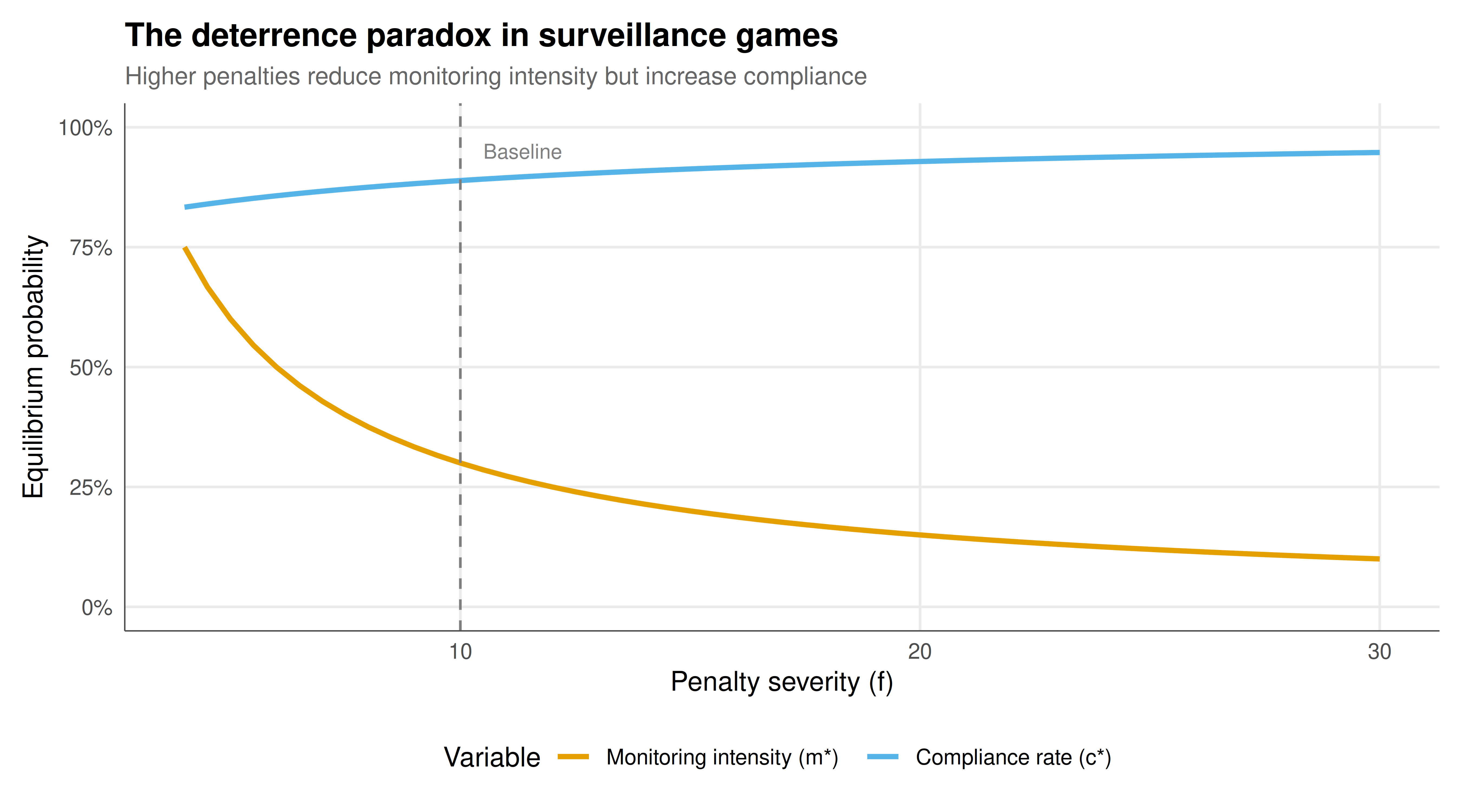
#| fig-cap: "Equilibrium monitoring intensity and citizen compliance rate as functions of penalty severity, illustrating the deterrence paradox: increasing penalties reduce equilibrium surveillance intensity while raising compliance. The vertical dashed line marks the baseline penalty. Okabe-Ito palette."
#| dev: [png, pdf]
#| dpi: 300
#| fig-width: 9
#| fig-height: 5
plot_df <- comparative_df %>%
  select(penalty, m_star, c_star) %>%
  pivot_longer(cols = c(m_star, c_star),
               names_to = "variable", values_to = "value") %>%
  mutate(variable = factor(variable,
                           levels = c("m_star", "c_star"),
                           labels = c("Monitoring intensity (m*)",
                                      "Compliance rate (c*)")))

p_static <- ggplot(plot_df, aes(x = penalty, y = value, color = variable)) +
  geom_line(linewidth = 1.1) +
  geom_vline(xintercept = f, linetype = "dashed", color = "grey50") +
  annotate("text", x = f + 0.5, y = 0.95, label = "Baseline",
           hjust = 0, size = 3.2, color = "grey50") +
  scale_color_manual(values = okabe_ito[1:2]) +
  scale_y_continuous(labels = scales::percent_format(), limits = c(0, 1)) +
  labs(title = "The deterrence paradox in surveillance games",
       subtitle = "Higher penalties reduce monitoring intensity but increase compliance",
       x = "Penalty severity (f)",
       y = "Equilibrium probability",
       color = "Variable") +
  theme_publication()

p_static
```
## Interactive figure
```{r}
#| label: fig-surveillance-interactive
#| fig-cap: "Interactive visualization of equilibrium outcomes and welfare as functions of penalty severity. Hover to see exact values for monitoring intensity, compliance rate, and total welfare at each penalty level."
welfare_plot_df <- comparative_df %>%
  select(penalty, m_star, c_star, welfare) %>%
  pivot_longer(cols = c(m_star, c_star, welfare),
               names_to = "variable", values_to = "value") %>%
  mutate(
    variable = factor(variable,
                      levels = c("m_star", "c_star", "welfare"),
                      labels = c("Monitoring (m*)", "Compliance (c*)", "Welfare")),
    text = paste0("Penalty: ", round(penalty, 1),
                  "\n", variable, ": ", round(value, 3))
  )

p_int <- ggplot(welfare_plot_df, aes(x = penalty, y = value,
                                      color = variable, text = text)) +
  geom_line(linewidth = 0.8) +
  scale_color_manual(values = okabe_ito[1:3]) +
  labs(title = "Surveillance equilibrium: comparative statics",
       x = "Penalty severity (f)",
       y = "Value",
       color = "Variable") +
  theme_publication()

ggplotly(p_int, tooltip = "text") |>
  config(displaylogo = FALSE,
         modeBarButtonsToRemove = c("select2d", "lasso2d"))
```
## Interpretation
The surveillance-privacy equilibrium model reveals several counterintuitive insights that have direct implications for policy design. The most striking result is the deterrence paradox: in the mixed-strategy equilibrium, increasing the penalty for detected violations does not increase the equilibrium monitoring intensity. Instead, it decreases it. The intuition is straightforward once the equilibrium logic is understood. The monitoring intensity is set to make the citizen indifferent between complying and violating. When penalties increase, the citizen needs to face a lower probability of detection to remain indifferent -- so the authority monitors less. Conversely, the compliance rate increases because higher penalties require fewer violations to keep the authority indifferent about the cost of monitoring.
This result has profound implications for surveillance policy. Policymakers who advocate for harsher penalties as a deterrent may be surprised to find that the equilibrium response involves reduced monitoring effort. In practical terms, this means that a society with very harsh penalties but low monitoring intensity may be indistinguishable in its compliance outcomes from a society with moderate penalties and moderate monitoring. The equilibrium compliance rate $c^* = 1 - k/(d + f)$ increases with the penalty $f$, so harsher penalties do improve compliance -- but through a mechanism that simultaneously reduces the authority's investment in surveillance infrastructure.
The welfare analysis adds another important dimension. Total equilibrium welfare is negative and depends on both the monitoring cost and the penalty structure. As penalties increase beyond a certain threshold, the marginal welfare gains from improved compliance diminish while the fixed costs of maintaining the monitoring apparatus remain. This suggests the existence of an optimal penalty level that balances deterrence effectiveness against the social costs of the surveillance infrastructure required to support it.
From a privacy perspective, the model highlights that citizens' equilibrium behavior is fundamentally shaped by the surveillance parameters. When monitoring costs decrease -- as has occurred dramatically with digital surveillance technologies -- the equilibrium shifts toward higher compliance but also higher monitoring intensity. This formalization captures the often-expressed concern that cheaper surveillance leads to more surveillance, even when the absolute level of non-compliance is low. The welfare implications of this shift are ambiguous: reduced violations benefit society, but increased monitoring imposes direct costs and may erode the value of privacy itself, a factor not fully captured in the basic model.
The inspection game framework also illuminates the role of commitment and transparency in surveillance policy. In the simultaneous-move game analyzed here, both players randomize. However, if the authority could credibly commit to a monitoring schedule in advance (a Stackelberg leader model), it could potentially achieve a higher payoff by choosing a monitoring intensity that optimally deters violations while minimizing costs. This connection between commitment and improved outcomes in inspection games parallels the broader game-theoretic literature on the value of commitment and has practical implications for whether surveillance policies should be transparent or opaque.
Finally, it is important to acknowledge the limitations of the basic model. Real surveillance-privacy interactions involve asymmetric information about citizen types (some citizens never violate, others always do), repeated interactions with reputation effects, multiple authorities with overlapping jurisdictions, and rich social norms about privacy that are not easily captured by simple payoff functions. Nevertheless, the core inspection game model provides the essential strategic logic that underpins more elaborate analyses of surveillance policy.
## Extensions and related tutorials
- [Von Neumann's minimax theorem](../../history-of-gt-mathematics/von-neumann-minimax-proof/) -- the foundational result for zero-sum games, which inspection games extend to asymmetric monitoring settings.
- [Organ donation mechanism design](../../ethics-and-game-theory/organ-donation-mechanism/) -- another application of mechanism design to socially sensitive allocation problems.
- [Commitment schemes and strategic credibility](../../cryptography-and-gt/commitment-schemes-game-theory/) -- how cryptographic commitments can enable credible monitoring policies.
- [Instrumental variables in strategic settings](../../causal-inference/instrumental-variables-strategic/) -- econometric tools for estimating causal effects in games with endogenous actions.
## References
::: {#refs}
:::