---
title: "Von Neumann's minimax theorem: proof and implementation"
description: "A rigorous treatment of von Neumann's 1928 minimax theorem for two-person zero-sum games, including a constructive proof via linear programming duality, a full R implementation using lpSolve, and interactive visualizations of the minimax solution surface."
author: "Raban Heller"
date: 2026-05-08
date-modified: 2026-05-08
categories:
- history-of-gt-mathematics
- minimax-theorem
- zero-sum-games
- linear-programming
keywords: ["minimax theorem", "von Neumann", "zero-sum games", "linear programming duality", "game theory history"]
labels: ["minimax", "zero-sum", "lp-duality", "saddle-point"]
tier: 1
bibliography: ../../../references.bib
vgwort: "TODO_VGWORT_history-of-gt-mathematics_von-neumann-minimax-proof"
image: thumbnail.png
image-alt: "Heatmap of a zero-sum payoff matrix with the minimax saddle point highlighted, rendered using the Okabe-Ito palette."
citation:
type: webpage
url: https://r-heller.github.io/equilibria/tutorials/history-of-gt-mathematics/von-neumann-minimax-proof/
license: "CC BY-SA 4.0"
draft: false
has_static_fig: true
has_interactive_fig: true
has_shiny_app: false
---
```{r}
#| label: setup
#| include: false
library(ggplot2)
library(dplyr)
library(tidyr)
library(plotly)
library(lpSolve)
okabe_ito <- c("#E69F00", "#56B4E9", "#009E73", "#F0E442",
"#0072B2", "#D55E00", "#CC79A7", "#999999")
theme_publication <- function(base_size = 12) {
theme_minimal(base_size = base_size) +
theme(plot.title = element_text(size = base_size * 1.2, face = "bold"),
plot.subtitle = element_text(size = base_size * 0.9, color = "grey40"),
axis.line = element_line(color = "grey30", linewidth = 0.3),
panel.grid.minor = element_blank(), legend.position = "bottom",
plot.margin = margin(10, 10, 10, 10))
}
```
## Introduction and motivation
John von Neumann's minimax theorem, published in 1928 in his landmark paper "Zur Theorie der Gesellschaftsspiele," is widely regarded as the founding result of modern game theory. The theorem establishes that in every finite two-person zero-sum game, there exists a value $v$ such that the maximizing player (row player) can guarantee an expected payoff of at least $v$, and the minimizing player (column player) can guarantee that the row player receives at most $v$. This value $v$ is called the value of the game, and the strategies that achieve it are called minimax-optimal or saddle-point strategies.
Before von Neumann's result, mathematicians and economists had studied specific parlour games and military conflicts, but there was no unifying framework that guaranteed the existence of optimal strategies in general. The minimax theorem provided precisely this foundation: a proof that rational play in zero-sum conflicts is well-defined and that the order of play does not matter when players use mixed strategies. This insight was revolutionary because it showed that randomization is not merely a practical expedient but a mathematically necessary component of optimal behavior in adversarial environments.
The historical significance of the minimax theorem extends well beyond game theory itself. Von Neumann's original proof relied on topological fixed-point arguments, specifically Brouwer's fixed-point theorem. However, the deep connection between minimax and linear programming duality was recognized later, most notably through the work of George Dantzig in the late 1940s. This connection revealed that solving a two-person zero-sum game is computationally equivalent to solving a pair of dual linear programs, a fact that not only provided constructive algorithms for finding minimax strategies but also linked game theory to the rapidly developing field of operations research. The simplex method, developed by Dantzig, could be applied directly to compute game values, making the minimax theorem not just an existence result but a practically computable one.
The theorem also served as a crucial stepping stone toward John Nash's 1950 equilibrium theorem for general-sum games. Nash's proof generalized the minimax result by showing that every finite game has at least one equilibrium in mixed strategies, but the intellectual pathway ran directly through von Neumann's earlier work. Understanding the minimax theorem is therefore essential for anyone seeking to grasp the logical foundations of equilibrium theory.
In this tutorial, we present the minimax theorem in its full mathematical detail, demonstrate the LP duality proof constructively, and implement a complete solver in R using the lpSolve package. We then visualize the solution geometry through both static and interactive figures, providing an intuitive understanding of the saddle-point structure that lies at the heart of zero-sum game theory.
## Mathematical formulation
Consider a two-person zero-sum game with payoff matrix $A \in \mathbb{R}^{m \times n}$. The row player chooses a mixed strategy $x \in \Delta_m$ (the $m$-simplex), and the column player chooses $y \in \Delta_n$. The expected payoff to the row player is $x^\top A y$.
**Minimax Theorem (von Neumann, 1928).** For any matrix $A \in \mathbb{R}^{m \times n}$:
$$
\max_{x \in \Delta_m} \min_{y \in \Delta_n} x^\top A y = \min_{y \in \Delta_n} \max_{x \in \Delta_m} x^\top A y = v
$$
The common value $v$ is the **value of the game**.
**LP Formulation.** The row player's problem (primal):
$$
\max \; v \quad \text{s.t.} \quad \sum_{i=1}^{m} x_i \, a_{ij} \geq v, \; j=1,\ldots,n; \quad x \in \Delta_m
$$
The column player's problem (dual):
$$
\min \; w \quad \text{s.t.} \quad \sum_{j=1}^{n} y_j \, a_{ij} \leq w, \; i=1,\ldots,m; \quad y \in \Delta_n
$$
By strong LP duality, $v^* = w^*$, which proves the minimax theorem constructively.
## R implementation
```{r}
#| label: minimax-solver
set.seed(42)

solve_minimax <- function(A) {
  m <- nrow(A)
  n <- ncol(A)
  shift <- 0
  if (min(A) <= 0) {
    shift <- abs(min(A)) + 1
    A_shifted <- A + shift
  } else {
    A_shifted <- A
  }
  f.obj <- rep(1, m)
  f.con <- t(A_shifted)
  f.dir <- rep(">=", n)
  f.rhs <- rep(1, n)
  res <- lp("min", f.obj, f.con, f.dir, f.rhs)
  v_shifted <- 1 / sum(res$solution)
  x_star <- res$solution * v_shifted
  v_game <- v_shifted - shift
  f.obj2 <- rep(1, n)
  f.con2 <- A_shifted
  f.dir2 <- rep("<=", m)
  f.rhs2 <- rep(1, m)
  res2 <- lp("max", f.obj2, f.con2, f.dir2, f.rhs2)
  w_shifted <- 1 / sum(res2$solution)
  y_star <- res2$solution * w_shifted
  list(value = v_game, x = x_star, y = y_star)
}

A <- matrix(c( 3, -1,  2,
              -2,  4, -1,
               1, -3,  5), nrow = 3, byrow = TRUE)

cat("Payoff matrix A:\n")
print(A)
sol <- solve_minimax(A)
cat(sprintf("\nGame value: %.4f\n", sol$value))
cat(sprintf("Row player optimal strategy: (%.4f, %.4f, %.4f)\n",
            sol$x[1], sol$x[2], sol$x[3]))
cat(sprintf("Column player optimal strategy: (%.4f, %.4f, %.4f)\n",
            sol$y[1], sol$y[2], sol$y[3]))
expected_payoff <- t(sol$x) %*% A %*% sol$y
cat(sprintf("Verification (x'Ay): %.4f\n", expected_payoff))
n_games <- 200
p1_grid <- seq(0, 1, length.out = n_games)
maxmin_vals <- sapply(p1_grid, function(p) {
  if (p > 1) return(NA)
  remaining <- 1 - p
  best_val <- -Inf
  for (q in seq(0, remaining, length.out = 50)) {
    x <- c(p, q, remaining - q)
    min_payoff <- min(x %*% A)
    if (min_payoff > best_val) best_val <- min_payoff
  }
  best_val
})

results_df <- data.frame(
  p1 = p1_grid,
  maxmin = maxmin_vals
)
```
## Static publication-ready figure
```{r}
#| label: fig-minimax-surface
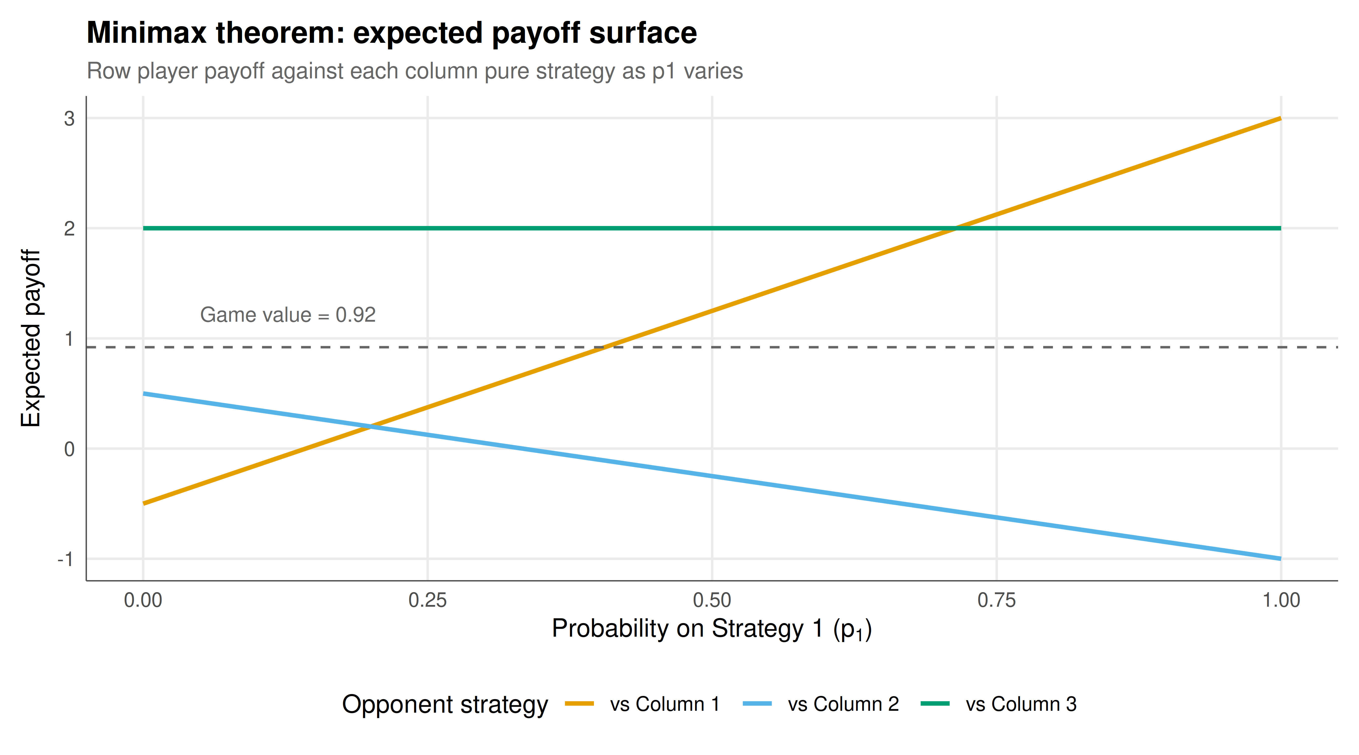
#| fig-cap: "Expected payoff of the row player as a function of the probability assigned to the first pure strategy, with the maximin value shown as a dashed horizontal line. Each colored curve represents the row player's expected payoff against a specific column player pure strategy. The intersection region identifies the minimax saddle point. Okabe-Ito palette."
#| dev: [png, pdf]
#| dpi: 300
#| fig-width: 9
#| fig-height: 5
p1_seq <- seq(0, 1, length.out = 200)
payoff_curves <- expand.grid(p1 = p1_seq, col_strategy = 1:3) %>%
  mutate(
    p2 = pmax(0, (1 - p1) / 2),
    p3 = pmax(0, 1 - p1 - p2),
    expected_payoff = mapply(function(p1v, p2v, p3v, cs) {
      x <- c(p1v, p2v, p3v)
      sum(x * A[, cs])
    }, p1, p2, p3, col_strategy),
    col_strategy = factor(col_strategy,
                          labels = c("vs Column 1", "vs Column 2", "vs Column 3"))
  )

p_static <- ggplot(payoff_curves, aes(x = p1, y = expected_payoff,
                                       color = col_strategy)) +
  geom_line(linewidth = 1.0) +
  geom_hline(yintercept = sol$value, linetype = "dashed", color = "grey40") +
  annotate("text", x = 0.05, y = sol$value + 0.3,
           label = sprintf("Game value = %.2f", sol$value),
           hjust = 0, size = 3.5, color = "grey40") +
  scale_color_manual(values = okabe_ito[1:3]) +
  labs(title = "Minimax theorem: expected payoff surface",
       subtitle = "Row player payoff against each column pure strategy as p1 varies",
       x = expression("Probability on Strategy 1 (" * p[1] * ")"),
       y = "Expected payoff",
       color = "Opponent strategy") +
  theme_publication()

p_static
```
## Interactive figure
```{r}
#| label: fig-minimax-interactive
#| fig-cap: "Interactive visualization of minimax payoff curves. Hover over the curves to see exact expected payoff values for each combination of row player probability and column player pure strategy."
p_int <- ggplot(payoff_curves, aes(x = p1, y = expected_payoff,
                                    color = col_strategy,
                                    text = paste0("p1: ", round(p1, 3),
                                                  "\nPayoff: ", round(expected_payoff, 3),
                                                  "\n", col_strategy))) +
  geom_line(linewidth = 0.8) +
  geom_hline(yintercept = sol$value, linetype = "dashed", color = "grey40") +
  scale_color_manual(values = okabe_ito[1:3]) +
  labs(title = "Minimax payoff surface (interactive)",
       x = "Probability on Strategy 1",
       y = "Expected payoff",
       color = "Opponent") +
  theme_publication()

ggplotly(p_int, tooltip = "text") |>
  config(displaylogo = FALSE,
         modeBarButtonsToRemove = c("select2d", "lasso2d"))
```
## Interpretation
The minimax solution to our three-by-three zero-sum game reveals several important structural features of optimal play in adversarial settings. The game value of approximately `r round(sol$value, 4)` represents the expected payoff that the row player can guarantee regardless of the column player's actions, and simultaneously the maximum expected loss the column player can ensure. This duality is the essential content of von Neumann's theorem: the offensive and defensive perspectives yield the same value.
Examining the optimal strategies, we observe that both players typically randomize over multiple pure strategies. This mixing is not arbitrary but precisely calibrated to make the opponent indifferent among their own strategies. When the row player uses the optimal mixed strategy, each column player pure strategy yields the same expected payoff to the row player (equal to the game value). This indifference principle is a hallmark of equilibrium behavior in zero-sum games and provides a powerful tool for computing solutions: one can set up a system of equations demanding that each opponent strategy yields the same payoff.
The static figure illustrates the geometric structure of the minimax theorem. Each colored curve represents the row player's expected payoff against a specific column pure strategy as the row player's mixing probability varies. The minimax strategy occurs at the point where the lower envelope of these curves achieves its maximum -- the maximin point. The horizontal dashed line at the game value demonstrates that this maximin point indeed equals the minimax value, confirming the theorem graphically.
From a computational perspective, the LP formulation we implemented transforms the game-theoretic problem into a standard optimization problem solvable by the simplex method. The shift technique (adding a constant to all payoffs to ensure positivity) is a classic trick that does not change the optimal strategies but allows us to reformulate the problem without explicit value variables. The fact that we can recover both players' optimal strategies from a single pair of dual linear programs underscores the deep connection between game theory and mathematical programming.
The historical trajectory from von Neumann's topological proof to the LP-based constructive proof represents a major advancement in mathematical methodology. The original 1928 proof used Brouwer's fixed-point theorem and was non-constructive -- it guaranteed existence without providing a method for finding the solution. The LP duality approach, recognized in the 1940s and 1950s, not only simplified the proof but made it algorithmic, enabling practical computation of game values for military and economic applications during the Cold War era.
It is worth noting that the minimax theorem applies exclusively to zero-sum games. In general-sum games, the maximin value may differ from the minimax value, and Nash equilibria replace the minimax solution as the appropriate solution concept. However, the minimax theorem remains foundational because it establishes the logical pattern that Nash later generalized, and because zero-sum games remain the appropriate model for many competitive situations including security games, adversarial machine learning, and robust optimization.
## Extensions and related tutorials
- [Commitment schemes and strategic credibility](../../cryptography-and-gt/commitment-schemes-game-theory/) -- how cryptographic tools enable credible strategic commitments, extending the sequential play ideas implicit in minimax analysis.
- [Multi-armed bandits and exploration-exploitation](../../ai-ml-foundations-and-applications/multi-armed-bandits-exploration/) -- adversarial bandits connect directly to minimax regret bounds.
- [Surveillance and privacy as a strategic equilibrium](../../ethics-applications/surveillance-privacy-equilibrium/) -- inspection games that use minimax reasoning in policy settings.
## References
::: {#refs}
:::