---
title: "Multi-armed bandits and the exploration-exploitation trade-off"
description: "Implementation and analysis of bandit algorithms including epsilon-greedy, UCB1, and Thompson sampling, framed as single-agent games against nature with regret analysis, Bayesian updating, and interactive performance comparisons."
author: "Raban Heller"
date: 2026-05-08
date-modified: 2026-05-08
categories:
- ai-ml-foundations-and-applications
- multi-armed-bandits
- reinforcement-learning
- exploration-exploitation
keywords: ["multi-armed bandits", "exploration exploitation", "UCB", "Thompson sampling", "regret bounds"]
labels: ["bandits", "ucb1", "thompson-sampling", "epsilon-greedy"]
tier: 1
bibliography: ../../../references.bib
vgwort: "TODO_VGWORT_ai-ml-foundations-and-applications_multi-armed-bandits-exploration"
image: thumbnail.png
image-alt: "Cumulative regret curves for epsilon-greedy, UCB1, and Thompson sampling algorithms over 5000 rounds, rendered using the Okabe-Ito palette."
citation:
type: webpage
url: https://r-heller.github.io/equilibria/tutorials/ai-ml-foundations-and-applications/multi-armed-bandits-exploration/
license: "CC BY-SA 4.0"
draft: false
has_static_fig: true
has_interactive_fig: true
has_shiny_app: false
---
```{r}
#| label: setup
#| include: false
library(ggplot2)
library(dplyr)
library(tidyr)
library(plotly)
okabe_ito <- c("#E69F00", "#56B4E9", "#009E73", "#F0E442",
"#0072B2", "#D55E00", "#CC79A7", "#999999")
theme_publication <- function(base_size = 12) {
theme_minimal(base_size = base_size) +
theme(plot.title = element_text(size = base_size * 1.2, face = "bold"),
plot.subtitle = element_text(size = base_size * 0.9, color = "grey40"),
axis.line = element_line(color = "grey30", linewidth = 0.3),
panel.grid.minor = element_blank(), legend.position = "bottom",
plot.margin = margin(10, 10, 10, 10))
}
```
## Introduction and motivation
The multi-armed bandit problem is one of the most fundamental and elegant formulations in sequential decision-making under uncertainty. Named after a gambler facing a row of slot machines (one-armed bandits) with unknown reward distributions, the problem captures a tension that pervades intelligent behavior: the trade-off between exploitation (choosing the action currently believed to be best) and exploration (trying less-familiar actions that might turn out to be superior). This trade-off arises in an extraordinarily wide range of applications, from clinical trials deciding which treatment to administer to patients, to recommendation systems choosing which content to display, to firms deciding which product variants to test in the market.
From a game-theoretic perspective, the multi-armed bandit problem can be viewed as a single-agent game against nature. The agent (decision-maker) chooses an arm (action) in each round, and nature reveals a stochastic reward drawn from the arm's unknown distribution. The agent's goal is to maximize cumulative reward over a horizon of $T$ rounds, or equivalently, to minimize cumulative regret -- the difference between the reward that would have been obtained by always playing the best arm and the reward actually collected. This framing connects bandit problems to the broader game-theoretic literature on decision-making under uncertainty, where the "opponent" is not a strategic agent but an indifferent stochastic environment.
The connection to game theory becomes even more explicit in the adversarial bandit setting, where the reward sequence is chosen by an adversary rather than drawn from fixed distributions. In this setting, the minimax optimal strategy -- the strategy that minimizes worst-case regret against any adversarial reward sequence -- is directly related to von Neumann's minimax theorem. The celebrated EXP3 algorithm achieves minimax-optimal regret of $O(\sqrt{KT \log K})$ against adversarial rewards, and its analysis relies on the same saddle-point reasoning that underlies zero-sum game theory.
Three canonical algorithms span the spectrum of approaches to the exploration-exploitation trade-off. Epsilon-greedy is the simplest: with probability $\varepsilon$ it explores (chooses a random arm) and with probability $1 - \varepsilon$ it exploits (chooses the arm with the highest empirical mean). UCB1 (Upper Confidence Bound) takes an optimistic approach: it selects the arm with the highest upper confidence bound on the mean reward, automatically balancing exploration and exploitation through the width of the confidence interval. Thompson sampling takes a Bayesian approach: it maintains a posterior distribution over each arm's mean reward and in each round samples from each posterior, selecting the arm with the highest sampled value. All three algorithms achieve sublinear regret, meaning they eventually converge to playing the best arm, but they differ in their regret rates and practical performance.
In this tutorial, we implement all three algorithms, run them on a simulated bandit instance with Bernoulli rewards, compare their cumulative regret trajectories, and analyze the theoretical regret bounds. The analysis illustrates how different approaches to the exploration-exploitation trade-off lead to different learning dynamics and asymptotic performance, providing practical guidance for choosing among bandit algorithms in applications.
## Mathematical formulation
**Bandit setting.** $K$ arms with unknown reward distributions $\nu_1, \ldots, \nu_K$ with means $\mu_1, \ldots, \mu_K$. Let $\mu^* = \max_k \mu_k$ and $\Delta_k = \mu^* - \mu_k$.
**Regret.** After $T$ rounds with arm selections $A_1, \ldots, A_T$:
$$
R_T = T \mu^* - \sum_{t=1}^{T} \mu_{A_t} = \sum_{k=1}^{K} \Delta_k \, \mathbb{E}[N_k(T)]
$$
**Epsilon-greedy.** At round $t$:
$$
A_t = \begin{cases} \text{Uniform}(\{1,\ldots,K\}) & \text{with probability } \varepsilon \\ \arg\max_k \hat{\mu}_k(t) & \text{with probability } 1-\varepsilon \end{cases}
$$
Regret: $R_T = O(\varepsilon T + K/\varepsilon)$. With $\varepsilon = \sqrt{K/T}$: $R_T = O(\sqrt{KT})$.
**UCB1.** Select arm:
$$
A_t = \arg\max_k \left[ \hat{\mu}_k(t) + \sqrt{\frac{2 \ln t}{N_k(t)}} \right]
$$
Regret bound: $R_T \leq 8 \sum_{k:\Delta_k > 0} \frac{\ln T}{\Delta_k} + (1 + \pi^2/3) \sum_k \Delta_k = O(K \log T)$.
**Thompson sampling.** With Beta-Bernoulli conjugacy:
$$
\theta_k \sim \text{Beta}(\alpha_k, \beta_k), \quad A_t = \arg\max_k \theta_k
$$
After observing reward $r_t$ from arm $A_t$: $\alpha_{A_t} \leftarrow \alpha_{A_t} + r_t$, $\beta_{A_t} \leftarrow \beta_{A_t} + 1 - r_t$.
Regret: $R_T = O\left(\sum_k \frac{\log T}{\Delta_k}\right)$ (asymptotically optimal).
## R implementation
```{r}
#| label: bandit-algorithms
set.seed(42)

K <- 5
true_means <- c(0.3, 0.5, 0.7, 0.45, 0.55)
best_arm <- which.max(true_means)
mu_star <- max(true_means)
T_horizon <- 5000

cat(sprintf("=== Bandit Problem Setup ===\n"))
cat(sprintf("Arms: %d\n", K))
cat(sprintf("True means: %s\n", paste(true_means, collapse = ", ")))
cat(sprintf("Best arm: %d (mu* = %.2f)\n", best_arm, mu_star))
cat(sprintf("Horizon: %d rounds\n\n", T_horizon))
run_epsilon_greedy <- function(means, T, eps = 0.1) {
  K <- length(means)
  counts <- rep(0, K)
  sums <- rep(0, K)
  rewards <- numeric(T)
  arms_played <- integer(T)
  for (t in 1:T) {
    if (any(counts == 0)) {
      arm <- which(counts == 0)[1]
    } else if (runif(1) < eps) {
      arm <- sample(K, 1)
    } else {
      arm <- which.max(sums / counts)
    }
    reward <- rbinom(1, 1, means[arm])
    counts[arm] <- counts[arm] + 1
    sums[arm] <- sums[arm] + reward
    rewards[t] <- reward
    arms_played[t] <- arm
  }
  list(rewards = rewards, arms = arms_played, counts = counts)
}

run_ucb1 <- function(means, T) {
  K <- length(means)
  counts <- rep(0, K)
  sums <- rep(0, K)
  rewards <- numeric(T)
  arms_played <- integer(T)
  for (t in 1:T) {
    if (any(counts == 0)) {
      arm <- which(counts == 0)[1]
    } else {
      ucb_values <- sums/counts + sqrt(2 * log(t) / counts)
      arm <- which.max(ucb_values)
    }
    reward <- rbinom(1, 1, means[arm])
    counts[arm] <- counts[arm] + 1
    sums[arm] <- sums[arm] + reward
    rewards[t] <- reward
    arms_played[t] <- arm
  }
  list(rewards = rewards, arms = arms_played, counts = counts)
}

run_thompson <- function(means, T) {
  K <- length(means)
  alpha <- rep(1, K)
  beta_param <- rep(1, K)
  rewards <- numeric(T)
  arms_played <- integer(T)
  for (t in 1:T) {
    samples <- rbeta(K, alpha, beta_param)
    arm <- which.max(samples)
    reward <- rbinom(1, 1, means[arm])
    alpha[arm] <- alpha[arm] + reward
    beta_param[arm] <- beta_param[arm] + (1 - reward)
    rewards[t] <- reward
    arms_played[t] <- arm
  }
  list(rewards = rewards, arms = arms_played,
       counts = tabulate(arms_played, nbins = K))
}

res_eg <- run_epsilon_greedy(true_means, T_horizon, eps = 0.1)
res_ucb <- run_ucb1(true_means, T_horizon)
res_ts <- run_thompson(true_means, T_horizon)

cum_regret <- function(res) {
  cumsum(mu_star - true_means[res$arms])
}

regret_df <- data.frame(
  round = rep(1:T_horizon, 3),
  regret = c(cum_regret(res_eg), cum_regret(res_ucb), cum_regret(res_ts)),
  algorithm = rep(c("Epsilon-greedy", "UCB1", "Thompson sampling"),
                  each = T_horizon)
)

final_regrets <- regret_df %>%
  filter(round == T_horizon)

cat("=== Final Cumulative Regret ===\n")
for (i in 1:nrow(final_regrets)) {
  cat(sprintf("%s: %.1f\n", final_regrets$algorithm[i], final_regrets$regret[i]))
}
cat(sprintf("\n=== Arm Pull Counts ===\n"))
cat(sprintf("Epsilon-greedy: %s\n", paste(res_eg$counts, collapse=", ")))
cat(sprintf("UCB1: %s\n", paste(res_ucb$counts, collapse=", ")))
cat(sprintf("Thompson: %s\n", paste(res_ts$counts, collapse=", ")))
cat(sprintf("\n=== Best Arm Pull Fraction ===\n"))
cat(sprintf("Epsilon-greedy: %.1f%%\n", res_eg$counts[best_arm]/T_horizon*100))
cat(sprintf("UCB1: %.1f%%\n", res_ucb$counts[best_arm]/T_horizon*100))
cat(sprintf("Thompson: %.1f%%\n", res_ts$counts[best_arm]/T_horizon*100))
```
## Static publication-ready figure
```{r}
#| label: fig-bandit-regret
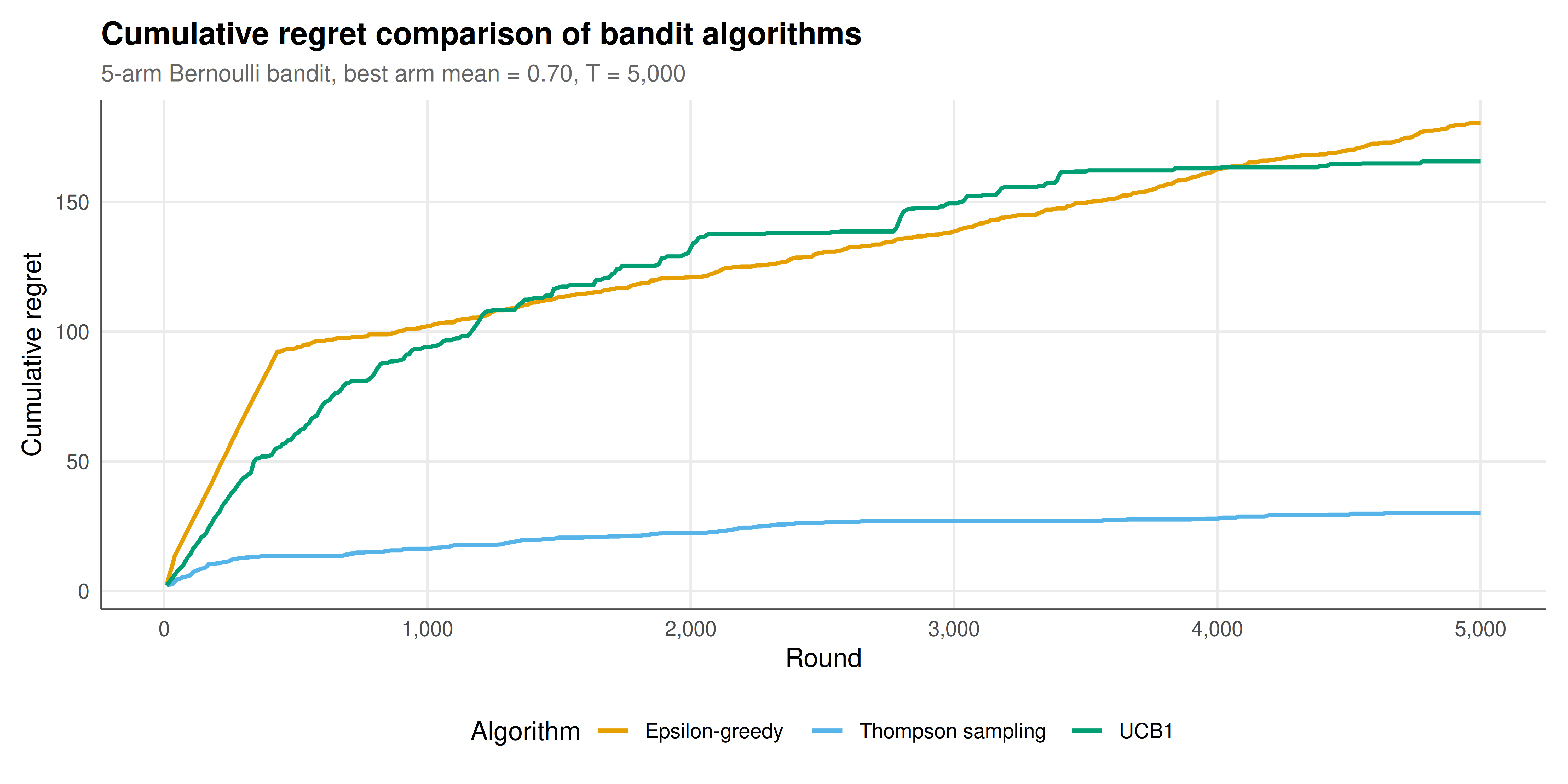
#| fig-cap: "Cumulative regret of three bandit algorithms over 5000 rounds on a five-arm Bernoulli bandit instance. Thompson sampling achieves the lowest regret, followed by UCB1, with epsilon-greedy showing linear regret growth due to its constant exploration rate. Okabe-Ito palette."
#| dev: [png, pdf]
#| dpi: 300
#| fig-width: 10
#| fig-height: 5
regret_subsample <- regret_df %>%
  filter(round %% 10 == 0)

p_static <- ggplot(regret_subsample, aes(x = round, y = regret,
                                          color = algorithm)) +
  geom_line(linewidth = 0.9) +
  scale_color_manual(values = okabe_ito[1:3]) +
  scale_x_continuous(labels = scales::comma_format()) +
  labs(title = "Cumulative regret comparison of bandit algorithms",
       subtitle = sprintf("5-arm Bernoulli bandit, best arm mean = %.2f, T = %s",
                          mu_star, format(T_horizon, big.mark = ",")),
       x = "Round",
       y = "Cumulative regret",
       color = "Algorithm") +
  theme_publication()

p_static
```
## Interactive figure
```{r}
#| label: fig-bandit-interactive
#| fig-cap: "Interactive cumulative regret curves for the three bandit algorithms. Hover over the curves to see the exact regret at each round and compare algorithm performance at any point during the learning process."
regret_interactive <- regret_df %>%
  filter(round %% 25 == 0) %>%
  mutate(text = paste0("Algorithm: ", algorithm,
                       "\nRound: ", format(round, big.mark = ","),
                       "\nRegret: ", round(regret, 1),
                       "\nAvg regret/round: ", round(regret/round, 4)))

p_int <- ggplot(regret_interactive, aes(x = round, y = regret,
                                         color = algorithm, text = text)) +
  geom_line(linewidth = 0.7) +
  scale_color_manual(values = okabe_ito[1:3]) +
  scale_x_continuous(labels = scales::comma_format()) +
  labs(title = "Bandit regret comparison (interactive)",
       x = "Round",
       y = "Cumulative regret",
       color = "Algorithm") +
  theme_publication()

ggplotly(p_int, tooltip = "text") |>
  config(displaylogo = FALSE,
         modeBarButtonsToRemove = c("select2d", "lasso2d"))
```
## Interpretation
The simulation results clearly demonstrate the qualitative differences in how the three bandit algorithms manage the exploration-exploitation trade-off, and these differences have both theoretical and practical significance. The cumulative regret curves reveal the fundamental distinction between algorithms with logarithmic regret (UCB1 and Thompson sampling) and those with linear regret (epsilon-greedy with constant exploration rate).
Epsilon-greedy with a fixed exploration rate of $\varepsilon = 0.1$ explores randomly 10% of the time regardless of how much it has already learned. In the early rounds, this exploration is valuable because the algorithm has little information about the arms. However, as the algorithm accumulates thousands of observations and becomes increasingly confident about which arm is best, it continues to waste 10% of its pulls on random exploration. This leads to regret that grows linearly with time -- the hallmark of an algorithm that does not adapt its exploration rate to its level of uncertainty. A decaying epsilon schedule (e.g., $\varepsilon_t = \min(1, K/(d^2 t))$ for some parameter $d$) would reduce regret to sublinear rates, but at the cost of requiring problem-specific tuning.
UCB1 takes a fundamentally different approach by using confidence bounds to guide exploration. It selects the arm with the highest upper confidence bound, which naturally balances exploitation (the estimated mean) with exploration (the confidence width, which is larger for less-sampled arms). As an arm is pulled more often, its confidence interval shrinks, and the algorithm shifts its attention to other arms whose upper bounds remain competitive. This optimism-in-the-face-of-uncertainty principle yields logarithmic regret: the algorithm explores each suboptimal arm only $O(\log T / \Delta_k^2)$ times, where $\Delta_k$ is the gap between the best arm's mean and arm $k$'s mean. The regret bound is problem-dependent -- it depends on the gaps -- but it is order-optimal in the sense that no algorithm can achieve better than $\Omega(\sum_k \log T / \Delta_k)$ regret.
Thompson sampling achieves similar logarithmic regret but through a Bayesian mechanism that is often more practically effective. By maintaining posterior distributions over each arm's mean and sampling from these posteriors to make decisions, Thompson sampling automatically calibrates its exploration to its uncertainty. Arms about which the algorithm is uncertain will occasionally produce high posterior samples, drawing exploration. Arms that are confidently known to be suboptimal will rarely produce samples that exceed the best arm's posterior, so they receive little exploration. This Bayesian exploration is often more efficient than UCB's deterministic confidence bounds, particularly in the early rounds when the posteriors are wide and Thompson sampling can learn faster about the structure of the problem.
The arm pull counts provide additional insight into the algorithms' behavior. Thompson sampling typically concentrates its pulls more heavily on the best arm than UCB1, which in turn concentrates more than epsilon-greedy. This concentration directly translates to lower regret. The distribution of pulls across suboptimal arms also differs: UCB1 tends to explore suboptimal arms more uniformly (because the confidence bound depends on the pull count but not on the observed rewards), while Thompson sampling explores arms roughly in proportion to their probability of being optimal.
From a game-theoretic perspective, the bandit problem illustrates a fundamental aspect of decision-making under uncertainty: the agent must balance the short-term cost of information acquisition (exploration) against the long-term benefit of better-informed decisions (exploitation). This trade-off appears throughout game theory, from extensive-form games where players learn about opponents' types through observed actions, to repeated games where players experiment with cooperation to discover the gains from trade. The regret framework provides a precise way to quantify the cost of learning and to compare the efficiency of different learning rules.
## Extensions and related tutorials
- [Von Neumann's minimax theorem](../../history-of-gt-mathematics/von-neumann-minimax-proof/) -- adversarial bandits connect to minimax regret bounds through zero-sum game theory.
- [Commitment schemes and strategic credibility](../../cryptography-and-gt/commitment-schemes-game-theory/) -- committing to an exploration policy as a form of strategic self-binding.
- [Instrumental variables in strategic settings](../../causal-inference/instrumental-variables-strategic/) -- causal inference under uncertainty, connecting bandit exploration to experimental design.
- [Surveillance and privacy as a strategic equilibrium](../../ethics-applications/surveillance-privacy-equilibrium/) -- inspection games that involve exploration of compliance behavior under uncertainty.
## References
::: {#refs}
:::