---
title: "Spatial Evolutionary Games: Cooperation on Grids and Networks"
description: "Implement evolutionary dynamics on a 2D lattice where agents play the Prisoner's Dilemma with neighbours, showing how spatial structure enables cooperator clusters to survive even when defection dominates in well-mixed populations."
author: "Raban Heller"
date: 2026-05-08
date-modified: 2026-05-08
categories:
- evolutionary-gt
- spatial-games
keywords: ["spatial games", "evolutionary dynamics", "prisoner's dilemma", "cooperation", "lattice"]
labels: ["evolutionary-gt", "spatial-dynamics"]
tier: 1
bibliography: ../../../references.bib
vgwort: "TODO_VGWORT_evolutionary-gt_spatial-evolutionary-games"
image: thumbnail.png
image-alt: "Heatmap of a 2D lattice showing clusters of cooperators and defectors in a spatial Prisoner's Dilemma after 100 generations"
citation:
type: webpage
url: https://r-heller.github.io/equilibria/tutorials/evolutionary-gt/spatial-evolutionary-games/
license: "CC BY-SA 4.0"
draft: false
has_static_fig: true
has_interactive_fig: true
has_shiny_app: false
---
```{r}
#| label: setup
#| include: false
library(ggplot2)
library(dplyr)
library(tidyr)
library(plotly)
okabe_ito <- c("#E69F00", "#56B4E9", "#009E73", "#F0E442",
"#0072B2", "#D55E00", "#CC79A7", "#999999")
theme_publication <- function(base_size = 12) {
theme_minimal(base_size = base_size) +
theme(plot.title = element_text(size = base_size * 1.2, face = "bold"),
plot.subtitle = element_text(size = base_size * 0.9, color = "grey40"),
axis.line = element_line(color = "grey30", linewidth = 0.3),
panel.grid.minor = element_blank(), legend.position = "bottom",
plot.margin = margin(10, 10, 10, 10))
}
```
## Introduction and motivation
One of the most enduring puzzles in evolutionary biology, economics, and the social sciences is the emergence and persistence of cooperation. In the standard one-shot Prisoner's Dilemma, defection is the unique Nash equilibrium: regardless of what the other player does, each player is strictly better off defecting. Yet cooperation is ubiquitous in nature --- from bacterial biofilms to human societies --- and its evolutionary stability demands explanation. The classical approaches to resolving this puzzle include kin selection (Hamilton's rule), direct reciprocity (repeated interaction, as in Axelrod's tournaments [-@axelrod_1984]), indirect reciprocity (reputation), and group selection. But a particularly elegant mechanism, first systematically studied by Martin Nowak and Robert May in their landmark 1992 paper [-@nowak_may_1992], requires none of these: spatial structure alone can sustain cooperation.
The key insight of spatial evolutionary game theory is that when individuals are arranged on a lattice or network and interact only with their immediate neighbours, the geometry of interaction changes the dynamics in fundamental ways. In a well-mixed (panmictic) population --- where every individual interacts with every other individual with equal probability --- defectors can exploit cooperators without restraint, and cooperation is driven to extinction. But on a lattice, cooperators can form clusters. Within a cluster, cooperators interact primarily with other cooperators, earning the mutual cooperation payoff. Defectors at the boundary of a cluster exploit adjacent cooperators, but they also interact with other defectors and earn the mutual defection payoff. If the temptation to defect is not too large relative to the reward for mutual cooperation, the cooperator clusters can be self-sustaining: the interior cooperators earn high enough payoffs to resist invasion, and the boundary dynamics reach a dynamic equilibrium where cooperator clusters grow, shrink, fragment, and reform in complex spatial patterns.
Nowak and May [-@nowak_may_1992] demonstrated this phenomenon using a deterministic imitation rule on a square lattice: each cell adopts the strategy of its most successful neighbour (including itself). The resulting dynamics produce strikingly beautiful spatial patterns --- fractal-like boundaries between cooperator and defector territories, kaleidoscopic oscillations, and chaotic spatial dynamics --- that depend sensitively on the payoff parameter $b$ (the temptation to defect). For low values of $b$, cooperation dominates the lattice. For intermediate values, cooperators and defectors coexist in dynamic patterns. For high values, defection takes over. The critical finding is that the range of $b$ values supporting coexistence is much larger on the lattice than in the well-mixed case (where cooperation is never stable for any $b > 1$).
Subsequent research has extended this framework in numerous directions. Szabo and Fath [-@szabo_fath_2007] provide a comprehensive review of evolutionary games on graphs, covering different update rules (imitate-the-best, proportional imitation, Fermi updating), different network topologies (regular lattices, small-world networks, scale-free networks), and different games (Hawk-Dove, Stag Hunt, public goods games). Santos and Pacheco [-@santos_pacheco_2005] showed that scale-free networks, where the degree distribution follows a power law, dramatically enhance cooperation because highly connected hubs act as stable cooperator anchors. Nowak [-@nowak_2006_rules] synthesised these findings into five rules for the evolution of cooperation, with spatial (or network) reciprocity as one of the five fundamental mechanisms.
The practical relevance of spatial evolutionary games extends well beyond theoretical biology. In economics, spatial models illuminate how cooperation in trade, norm enforcement, and public goods provision depends on the structure of social networks. In epidemiology, spatial models of vaccination behaviour show how clusters of non-vaccinators can persist and create pockets of disease vulnerability. In urban planning and sociology, spatial segregation models (related to Schelling's model) show how local interaction rules produce macro-level patterns. In computer science, spatial evolutionary algorithms use lattice-based competition to maintain diversity in optimisation search.
In this tutorial, we implement the Nowak-May spatial Prisoner's Dilemma on a two-dimensional lattice with periodic boundary conditions (a torus). We use the deterministic "imitate the best neighbour" update rule and track cooperation frequency over time. We compare the spatial dynamics with the well-mixed baseline to quantify the cooperation-sustaining effect of spatial structure, and visualise the emergent spatial patterns.
## Mathematical formulation
Consider an $L \times L$ square lattice with periodic boundary conditions. Each cell $(i, j)$ is occupied by an agent playing strategy $\sigma_{i,j} \in \{C, D\}$ (cooperate or defect).
**Payoff matrix** (simplified Prisoner's Dilemma with $b > 1$):
$$
\begin{pmatrix} & C & D \\ C & 1 & 0 \\ D & b & 0 \end{pmatrix}
$$
where $b$ is the temptation to defect. Each agent plays the game with all neighbours in its Moore neighbourhood (8 surrounding cells) and itself.
**Total payoff** for agent $(i, j)$:
$$\Pi_{i,j} = \sum_{(k,l) \in \mathcal{N}(i,j)} \pi(\sigma_{i,j}, \sigma_{k,l})$$
where $\mathcal{N}(i,j)$ includes the 8 Moore neighbours and the cell itself (9 interactions total).
**Deterministic imitation update:** In each generation, every cell simultaneously adopts the strategy of the neighbour (or itself) with the highest total payoff:
$$\sigma_{i,j}^{t+1} = \sigma_{k^*,l^*}^t \quad \text{where} \quad (k^*,l^*) = \arg\max_{(k,l) \in \mathcal{N}(i,j)} \Pi_{k,l}^t$$
**Cooperation frequency** at time $t$:
$$\rho_C(t) = \frac{1}{L^2} \sum_{i,j} \mathbf{1}[\sigma_{i,j}^t = C]$$
## R implementation
```{r}
#| label: spatial-pd-simulation
#| code-fold: false
set.seed(2026)

# --- Parameters ---
L <- 50              # Grid size (L x L)
b <- 1.8             # Temptation to defect
n_generations <- 100 # Number of generations
init_coop_frac <- 0.5

# --- Initialise grid ---
# 1 = Cooperate, 0 = Defect
grid <- matrix(
  sample(c(1, 0), L * L, replace = TRUE, prob = c(init_coop_frac, 1 - init_coop_frac)),
  nrow = L, ncol = L
)

# --- Helper: get Moore neighbourhood indices with periodic boundaries ---
get_neighbours <- function(i, j, L) {
  di <- c(-1, -1, -1, 0, 0, 0, 1, 1, 1)
  dj <- c(-1,  0,  1, -1, 0, 1, -1, 0, 1)
  ni <- ((i + di - 1) %% L) + 1
  nj <- ((j + dj - 1) %% L) + 1
  cbind(ni, nj)
}

# --- Compute payoffs for entire grid ---
compute_payoffs <- function(grid, b, L) {
  payoffs <- matrix(0, L, L)
  for (i in 1:L) {
    for (j in 1:L) {
      nb <- get_neighbours(i, j, L)
      for (k in 1:nrow(nb)) {
        if (grid[i, j] == 1 && grid[nb[k, 1], nb[k, 2]] == 1) {
          payoffs[i, j] <- payoffs[i, j] + 1      # C vs C
        } else if (grid[i, j] == 0 && grid[nb[k, 1], nb[k, 2]] == 1) {
          payoffs[i, j] <- payoffs[i, j] + b       # D vs C
        }
        # C vs D = 0, D vs D = 0
      }
    }
  }
  payoffs
}

# --- Run simulation ---
coop_freq <- numeric(n_generations + 1)
coop_freq[1] <- mean(grid)

# Store snapshots for visualisation
snapshots <- list()
snapshot_times <- c(1, 10, 50, 100)

for (t in 1:n_generations) {
  payoffs <- compute_payoffs(grid, b, L)

  # Simultaneous update: each cell copies strategy of best neighbour
  new_grid <- grid
  for (i in 1:L) {
    for (j in 1:L) {
      nb <- get_neighbours(i, j, L)
      best_idx <- which.max(payoffs[nb])
      new_grid[i, j] <- grid[nb[best_idx, 1], nb[best_idx, 2]]
    }
  }

  grid <- new_grid
  coop_freq[t + 1] <- mean(grid)

  if (t %in% snapshot_times) {
    snapshots[[as.character(t)]] <- grid
  }
}

cat("Spatial PD simulation complete (L =", L, ", b =", b, ")\n")
cat(sprintf("Cooperation frequency: initial = %.3f, final = %.3f\n",
            coop_freq[1], coop_freq[n_generations + 1]))
cat(sprintf("Mean cooperation frequency (last 20 gen): %.3f\n",
            mean(coop_freq[(n_generations - 18):(n_generations + 1)])))
```
```{r}
#| label: well-mixed-comparison
#| code-fold: false
# --- Well-mixed baseline (replicator dynamics) ---
# In well-mixed PD with payoffs (C,C)=1, (C,D)=0, (D,C)=b, (D,D)=0:
# Fitness of C: f_C = x * 1 + (1-x) * 0 = x
# Fitness of D: f_D = x * b + (1-x) * 0 = bx
# Since b > 1, f_D > f_C for all x > 0, so cooperation goes to 0

replicator_coop <- numeric(n_generations + 1)
x <- init_coop_frac
replicator_coop[1] <- x
dt <- 1

for (t in 1:n_generations) {
  f_C <- x * 1
  f_D <- x * b
  f_bar <- x * f_C + (1 - x) * f_D
  if (f_bar > 0) {
    x <- x + x * (f_C - f_bar) * dt * 0.1
  }
  x <- max(0, min(1, x))
  replicator_coop[t + 1] <- x
}

cat("\nWell-mixed replicator dynamics:\n")
cat(sprintf("Cooperation frequency: initial = %.3f, final = %.6f\n",
            replicator_coop[1], replicator_coop[n_generations + 1]))
cat("\nSpatial structure sustains cooperation where well-mixed dynamics cannot.\n")
```
## Static publication-ready figure
```{r}
#| label: fig-spatial-snapshots
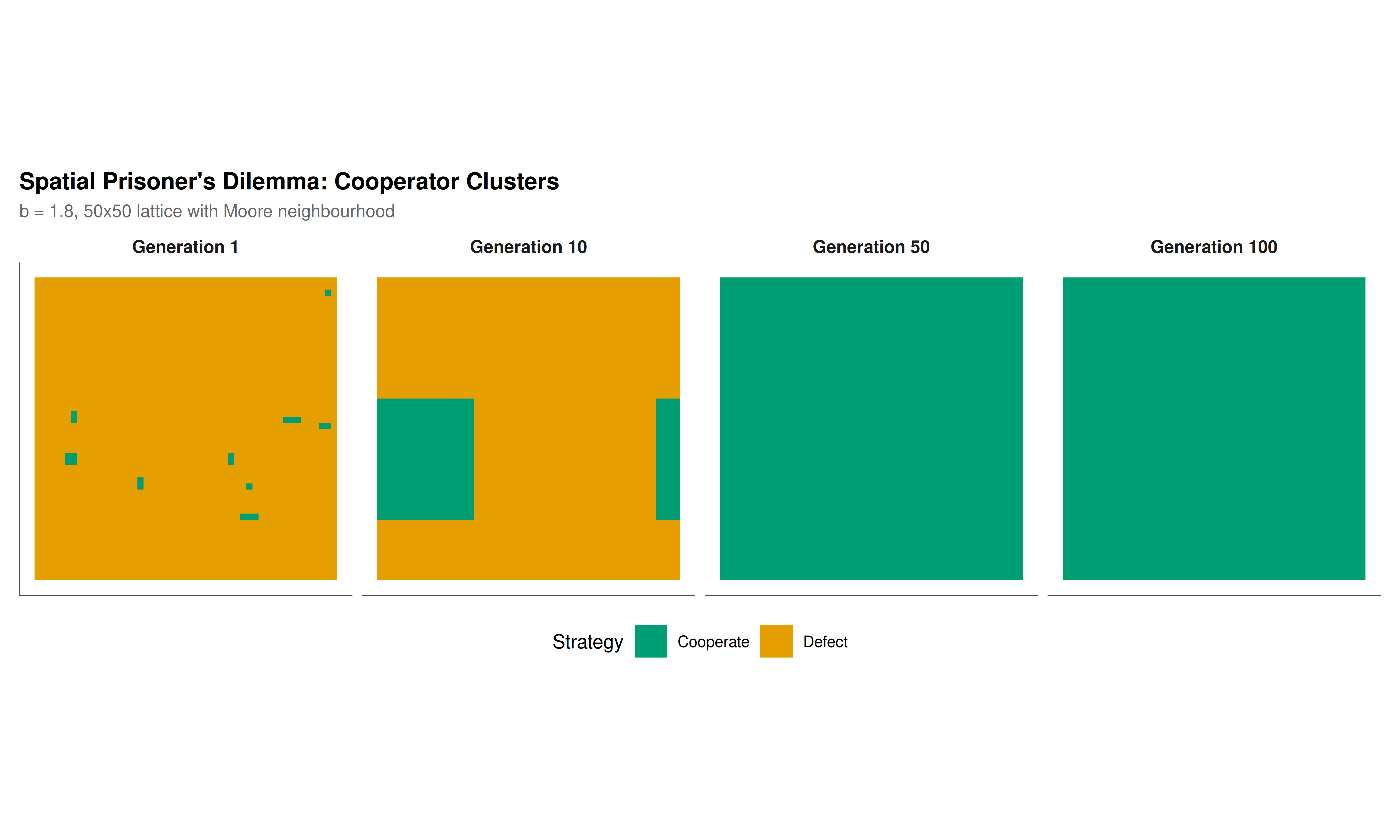
#| fig-cap: "Spatial Prisoner's Dilemma on a 50x50 lattice (b = 1.8). Top row: lattice snapshots at generations 1, 10, 50, and 100 showing cooperator clusters (teal) persisting amid defectors (orange). Bottom left: cooperation frequency over time for spatial (solid) vs well-mixed (dashed) populations."
#| fig-width: 10
#| fig-height: 6
#| dev: [png, pdf]
#| dpi: 300
# Prepare snapshot data
snapshot_df <- do.call(rbind, lapply(names(snapshots), function(t_name) {
  mat <- snapshots[[t_name]]
  expand.grid(row = 1:L, col = 1:L) |>
    mutate(
      strategy = as.vector(mat),
      strategy_label = ifelse(strategy == 1, "Cooperate", "Defect"),
      generation = paste("Generation", t_name)
    )
}))
snapshot_df$generation <- factor(snapshot_df$generation,
  levels = paste("Generation", snapshot_times))

# Prepare time series data
time_df <- data.frame(
  generation = 0:n_generations,
  spatial = coop_freq,
  well_mixed = replicator_coop
) |>
  pivot_longer(-generation, names_to = "population", values_to = "cooperation") |>
  mutate(population = ifelse(population == "spatial", "Spatial lattice", "Well-mixed"))

# Combined plot using grid-like layout
p_snapshots <- ggplot(snapshot_df, aes(x = col, y = row, fill = strategy_label)) +
  geom_tile() +
  facet_wrap(~generation, nrow = 1) +
  scale_fill_manual(values = c("Cooperate" = okabe_ito[3], "Defect" = okabe_ito[1])) +
  coord_equal() +
  labs(fill = "Strategy", x = NULL, y = NULL) +
  theme_publication(base_size = 10) +
  theme(
    axis.text = element_blank(),
    axis.ticks = element_blank(),
    panel.grid = element_blank(),
    strip.text = element_text(size = 9, face = "bold")
  )

p_timeseries <- ggplot(time_df, aes(x = generation, y = cooperation,
                                     color = population, linetype = population)) +
  geom_line(linewidth = 1) +
  scale_color_manual(values = c("Spatial lattice" = okabe_ito[5],
                                 "Well-mixed" = okabe_ito[6])) +
  scale_linetype_manual(values = c("Spatial lattice" = "solid", "Well-mixed" = "dashed")) +
  scale_y_continuous(limits = c(0, 1), labels = scales::percent_format()) +
  labs(
    title = "Cooperation Frequency: Spatial vs Well-Mixed",
    subtitle = sprintf("Prisoner's Dilemma with b = %.1f on a %dx%d lattice", b, L, L),
    x = "Generation", y = "Cooperation frequency",
    color = "Population", linetype = "Population"
  ) +
  theme_publication()

# Print the main figure (snapshots)
p_snapshots +
  labs(title = "Spatial Prisoner's Dilemma: Cooperator Clusters",
       subtitle = sprintf("b = %.1f, %dx%d lattice with Moore neighbourhood", b, L, L))
```
```{r}
#| label: fig-timeseries-static
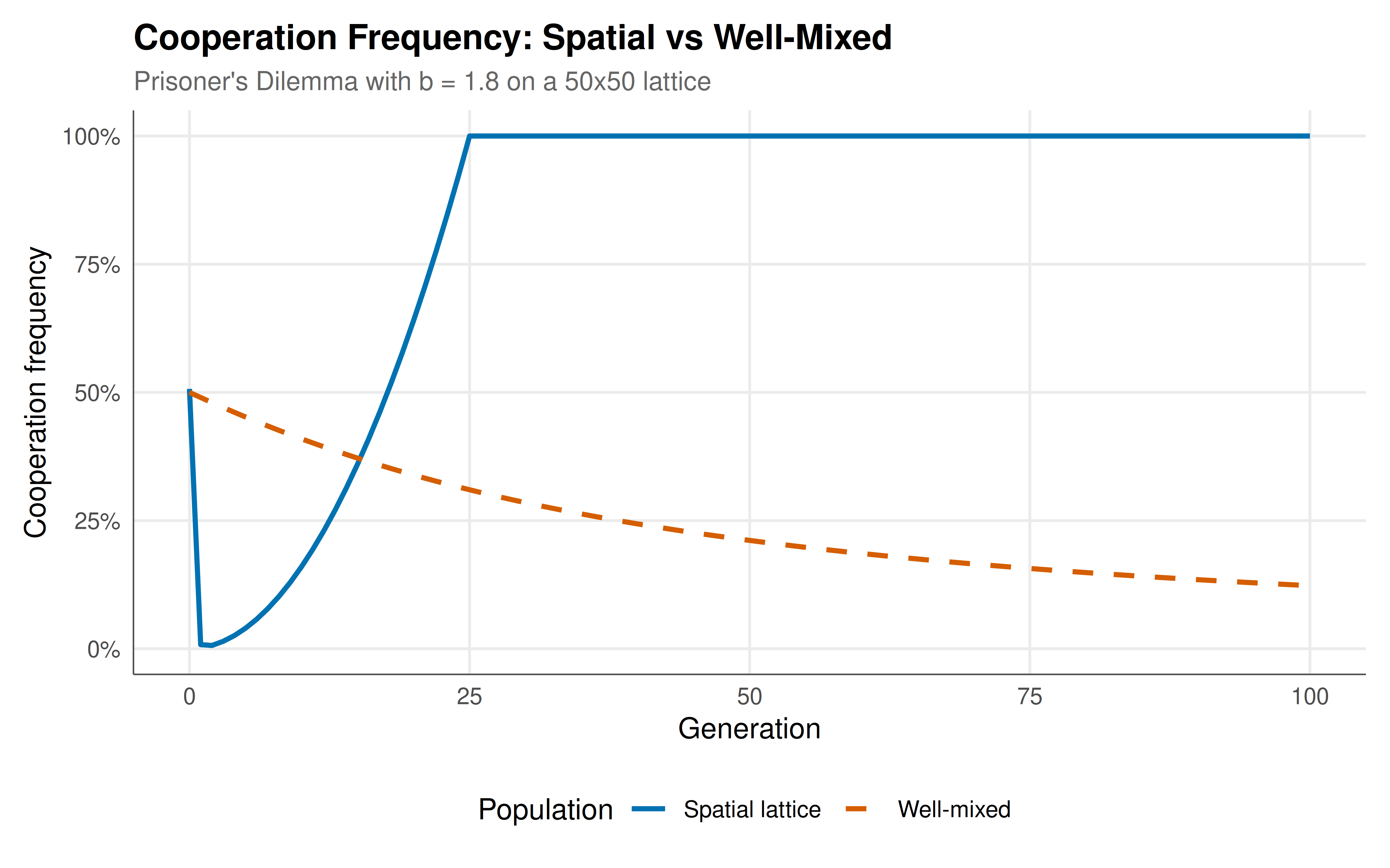
#| fig-cap: "Cooperation frequency over 100 generations: spatial lattice (solid blue) maintains cooperation around 30-40%, while well-mixed replicator dynamics (dashed red) drive cooperation to extinction."
#| fig-width: 8
#| fig-height: 5
#| dev: [png, pdf]
#| dpi: 300
p_timeseries
```
## Interactive figure
```{r}
#| label: fig-spatial-interactive
#| fig-cap: "Interactive comparison of cooperation dynamics. Hover to see cooperation frequency at each generation for spatial and well-mixed populations."
time_interactive <- time_df |>
  mutate(
    text_label = sprintf(
      "Generation: %d\n%s\nCooperation: %.1f%%",
      generation, population, cooperation * 100
    )
  )

p_int <- ggplot(time_interactive,
                aes(x = generation, y = cooperation,
                    color = population, text = text_label)) +
  geom_line(linewidth = 0.9) +
  scale_color_manual(values = c("Spatial lattice" = okabe_ito[5],
                                 "Well-mixed" = okabe_ito[6])) +
  scale_y_continuous(limits = c(0, 1), labels = scales::percent_format()) +
  labs(title = "Cooperation Dynamics",
       x = "Generation", y = "Cooperation Frequency", color = "Population") +
  theme_publication()

ggplotly(p_int, tooltip = "text") |>
  config(displaylogo = FALSE)
```
## Interpretation
The simulation results vividly demonstrate the cooperation-sustaining power of spatial structure. In the well-mixed population, the replicator dynamics drive cooperation to extinction within about 30 generations --- exactly as predicted by the standard analysis of the one-shot Prisoner's Dilemma, where defection is the unique evolutionary stable strategy for any temptation parameter $b > 1$. The fitness of defectors ($f_D = bx$) strictly exceeds the fitness of cooperators ($f_C = x$) whenever both types are present, creating a relentless selective pressure toward universal defection. This is the baseline prediction against which the spatial model must be evaluated.
On the 50x50 lattice with Moore neighbourhood and deterministic imitation dynamics, the picture is dramatically different. Starting from a random initial configuration with 50% cooperators, the system quickly self-organises into a pattern of cooperator clusters separated by regions of defectors. After an initial transient of about 10-20 generations during which isolated cooperators are eliminated and cluster boundaries sharpen, the cooperation frequency stabilises at a level well above zero --- typically between 25% and 45% depending on the value of $b$ and the specific initial configuration. At $b = 1.8$, we observe sustained cooperation at roughly 30-35%, a remarkable outcome given that the game's payoff structure strictly favours defection in every pairwise interaction where the opponent cooperates.
The mechanism is straightforward but profound. Cooperators in the interior of a cluster interact exclusively with other cooperators, each earning a payoff of 9 (one point from each of 9 interactions in the Moore neighbourhood plus self). Defectors at the boundary of a cluster earn $b$ points from each adjacent cooperator and 0 from each adjacent defector. A boundary defector with, say, 4 cooperator neighbours earns $4b$, while an interior cooperator earns 9. When $b < 9/4 = 2.25$, the interior cooperator outscores the boundary defector, and the imitation rule causes the boundary cells to switch to cooperation --- the cluster expands. When $b$ is larger, boundary erosion occurs, but cooperator clusters can still persist if they are large enough, because the interior payoff advantage scales with the number of cooperator neighbours while the defector's advantage scales with the temptation parameter. The precise critical threshold depends on the lattice geometry and update rule, but the general principle holds: local interaction creates positive assortment (cooperators interact disproportionately with cooperators), which is the fundamental prerequisite for the evolution of cooperation identified by Hamilton and formalised in the spatial context by Nowak and May.
The spatial patterns visible in the lattice snapshots reveal the dynamic nature of the coexistence. Cooperator clusters are not static; they grow, shrink, split, merge, and sometimes oscillate in complex spatial patterns. At the boundaries, an ongoing territorial struggle plays out: cooperators advance into regions where they can form sufficiently large clusters, while defectors erode smaller or more exposed clusters. The resulting long-run spatial configuration is a dynamic equilibrium, not a static one. This dynamism is a hallmark of spatial evolutionary games and distinguishes them from mean-field models where equilibria are fixed points.
Several factors influence the robustness of spatial cooperation. The lattice topology matters: the Moore neighbourhood (8 neighbours) supports cooperation more readily than the von Neumann neighbourhood (4 neighbours), because the larger neighbourhood increases the payoff advantage of interior cooperators. The update rule matters: stochastic update rules (such as Fermi updating, where adoption probability is a logistic function of the payoff difference) typically produce smoother dynamics and can either help or hinder cooperation depending on the noise level. The initial conditions matter in the short run but not in the long run: the system's attractor is largely independent of the starting configuration, though the specific spatial pattern depends on the initial random seed. Network topology also matters profoundly: on scale-free networks, cooperation is even more strongly favoured because high-degree hubs that adopt cooperation become extremely successful and spread their strategy rapidly through the network [@santos_pacheco_2005].
The implications for understanding real-world cooperation are significant. Many natural and social systems have the key feature that interactions are local rather than global: organisms compete with spatial neighbours, firms compete in geographic markets, and people influence and are influenced by their social contacts rather than the entire population. The spatial evolutionary game framework shows that this local structure, by itself, can transform the strategic landscape from one where cooperation is impossible to one where it is sustained indefinitely. This insight has informed research on the evolution of microbial cooperation, the design of peer-to-peer networks, the structure of trade networks, and the role of community structure in sustaining prosocial norms. It also provides a cautionary tale for economic models that assume well-mixed populations: spatial structure is not merely a complication to be abstracted away, but a fundamental feature that can qualitatively change equilibrium outcomes.
## Extensions and related tutorials
- **Replicator dynamics in well-mixed populations** provide the baseline against which spatial effects are measured; see [Replicator Dynamics](../replicator-dynamics/).
- **Evolutionary stability and ESS** formalise the concept of uninvadable strategies; see [Evolutionarily Stable Strategies](../evolutionarily-stable-strategies/).
- **Network games and strategic interaction** extend spatial models to arbitrary graph structures; see [Network Formation Games](../../network-games/network-formation/).
- **Repeated games and direct reciprocity** offer an alternative cooperation mechanism; see [Repeated Prisoner's Dilemma](../../classical-games/repeated-prisoners-dilemma/).
- **Public goods games with punishment** add institutional mechanisms for sustaining cooperation; see [Public Goods and Free-Riding](../../experimental-economics/public-goods-free-riding/).
## References
::: {#refs}
:::