---
title: "The p-beauty contest: level-k thinking and iterated dominance"
description: "Simulate the p-beauty contest guessing game to explore bounded rationality, level-k thinking, and the gap between Nash equilibrium predictions and experimental behaviour."
author: "Raban Heller"
date: 2026-05-08
date-modified: 2026-05-08
categories:
- experimental-economics
- bounded-rationality
- level-k-thinking
keywords: ["beauty contest", "guessing game", "level-k", "cognitive hierarchy", "bounded rationality", "R"]
labels: ["experimental", "behavioral"]
tier: 1
bibliography: ../../../references.bib
vgwort: "TODO_VGWORT_EXPERIMENTAL-ECONOMICS_BEAUTY-CONTEST-GUESSING"
image: thumbnail.png
image-alt: "Histogram of guesses in a p-beauty contest showing clusters at level-0, level-1, and level-2 thinking"
citation:
type: webpage
url: https://r-heller.github.io/equilibria/tutorials/experimental-economics/beauty-contest-guessing/
license: "CC BY-SA 4.0"
draft: false
has_static_fig: true
has_interactive_fig: true
has_shiny_app: false
---
```{r}
#| label: setup
#| include: false
library(ggplot2)
library(dplyr)
library(tidyr)
library(plotly)
okabe_ito <- c("#E69F00", "#56B4E9", "#009E73", "#F0E442",
"#0072B2", "#D55E00", "#CC79A7", "#999999")
theme_publication <- function(base_size = 12) {
theme_minimal(base_size = base_size) +
theme(plot.title = element_text(size = base_size * 1.2, face = "bold"),
plot.subtitle = element_text(size = base_size * 0.9, color = "grey40"),
axis.line = element_line(color = "grey30", linewidth = 0.3),
panel.grid.minor = element_blank(), legend.position = "bottom",
plot.margin = margin(10, 10, 10, 10))
}
```
## Introduction & motivation
The p-beauty contest, also known as the guessing game, is one of the most celebrated experiments in behavioural game theory. Named after a passage in John Maynard Keynes's *General Theory* (1936) comparing stock market speculation to a newspaper beauty contest where readers must guess which face other readers will choose as the most beautiful, the game strips strategic reasoning to its purest form. Each of $N$ players simultaneously chooses a number from the interval $[0, 100]$. The winner is the player whose guess is closest to $p$ times the mean of all guesses, where $p$ is a publicly known parameter typically set to $2/3$. The prize goes to the closest guess, with ties broken randomly. The game is simple to explain, easy to play, and yet it reveals profound truths about how people actually reason in strategic settings --- truths that standard game theory, with its assumption of perfect rationality, systematically misses [@nagel_1995].
The theoretical analysis of the game is straightforward via iterated elimination of dominated strategies. If all players are rational and believe others are rational, no one should guess above $100p$ (since the mean cannot exceed 100, the target cannot exceed $100p$). But if no one guesses above $100p$, then no one should guess above $100p^2$. Continuing this argument, the only strategy that survives infinite rounds of iterated dominance is 0. This is the unique Nash equilibrium of the game. Yet when the game is actually played --- in classrooms, in newspaper competitions, in laboratory experiments --- the number 0 is almost never chosen. Instead, guesses cluster around two characteristic values: approximately $100p/2 \approx 33$ (for $p = 2/3$), corresponding to one step of reasoning (level-1 thinking), and approximately $100p^2/2 \approx 22$, corresponding to two steps (level-2 thinking). The original experimental study by Rosemarie Nagel demonstrated this pattern convincingly, and it has been replicated hundreds of times across different populations and cultures.
The systematic departure from Nash equilibrium in the beauty contest motivated the development of the **level-k** model of strategic thinking [@stahl_wilson_1994; @costa_gomes_crawford_2006]. In this model, players are heterogeneous in their depth of reasoning. Level-0 players choose randomly (uniformly from $[0, 100]$). Level-1 players best-respond to level-0 play, choosing approximately $50p$. Level-2 players best-respond to level-1, choosing approximately $50p^2$. And so on. The population is a mixture of these types, with a distribution that can be estimated from experimental data. A related model, the **Cognitive Hierarchy** (CH) model of Camerer, Ho, and Chong [-@camerer_ho_chong_2004], refines this by assuming that each level-$k$ player best-responds to a Poisson-distributed mixture of all lower types, not just the level immediately below. The CH model typically fits experimental data better because it allows for a smooth distribution of thinking depths characterised by a single parameter $\tau$ (the mean of the Poisson distribution).
The beauty contest game has become a standard tool for measuring strategic sophistication across populations. Studies have compared the depth of reasoning in different groups --- economics students versus non-economists, CEOs versus college students, chess players versus laypeople --- and have consistently found that while depth of reasoning varies, even the most sophisticated populations rarely exhibit more than level-3 thinking in a one-shot game. The game has also been used to study learning dynamics: when the beauty contest is played repeatedly, guesses converge toward zero over time, but the speed of convergence depends on the value of $p$ and the group composition. This convergence pattern provides evidence for adaptive learning models where players gradually update their beliefs about others' behaviour.
Beyond its role in testing bounded rationality, the beauty contest connects to important questions in macroeconomics and finance. The Keynesian beauty contest metaphor captures the essence of speculative markets where traders must guess not what an asset is worth, but what other traders think it is worth. The information aggregation problem in financial markets has a beauty-contest structure, and models of expectation formation in macroeconomics (such as the "islands" model) exhibit similar dynamics. Understanding how real people reason about others' reasoning is thus not merely an academic exercise but has direct implications for understanding price formation, bubbles, and the effectiveness of central bank communication.
In this tutorial, we simulate the beauty contest with a population of heterogeneous level-k thinkers, implement the Poisson Cognitive Hierarchy model, compare the theoretical predictions with stylised patterns from experimental data, and explore how choices evolve over multiple rounds of play.
## Mathematical formulation
In the p-beauty contest, $N$ players each choose $x_i \in [0, 100]$. The target is $T = p \cdot \bar{x}$ where $\bar{x} = \frac{1}{N}\sum_{i=1}^N x_i$ and $0 < p < 1$. The winner is $\arg\min_i |x_i - T|$.
**Nash equilibrium.** The unique Nash equilibrium is $x_i^* = 0$ for all $i$, obtained by iterated elimination of dominated strategies.
**Level-k model.** Define the level-$k$ action recursively:
$$
x^{(0)} \sim \text{Uniform}(0, 100), \quad x^{(k)} = p \cdot \mathbb{E}[x^{(k-1)}]
$$
For the uniform level-0 anchor: $\mathbb{E}[x^{(0)}] = 50$, giving $x^{(1)} = 50p$, $x^{(2)} = 50p^2$, and in general $x^{(k)} = 50p^k$.
**Cognitive Hierarchy (CH) model.** The proportion of level-$k$ thinkers follows a Poisson distribution with mean $\tau$:
$$
f(k) = \frac{e^{-\tau} \tau^k}{k!}
$$
Each level-$k$ player best-responds to the mixture of levels $0, 1, \ldots, k-1$, weighted by their normalised proportions:
$$
g_k(h) = \frac{f(h)}{\sum_{m=0}^{k-1} f(m)}, \quad h = 0, 1, \ldots, k-1
$$
The level-$k$ action in the CH model is:
$$
x^{(k)}_{\text{CH}} = p \cdot \sum_{h=0}^{k-1} g_k(h) \cdot x^{(h)}_{\text{CH}}
$$
## R implementation
We implement both the level-k model and the Cognitive Hierarchy model, then simulate a multi-round beauty contest with adaptive learning.
```{r}
#| label: beauty-contest-implementation
set.seed(123)

p <- 2/3  # Beauty contest parameter
N <- 100  # Number of players

# --- Level-k predictions ---
level_k_action <- function(k, p) {
  if (k == 0) return(50)  # Expected value of Uniform(0, 100)
  50 * p^k
}

cat("=== Level-k predictions (p = 2/3) ===\n")
for (k in 0:6) {
  cat(sprintf("  Level-%d: %.2f\n", k, level_k_action(k, p)))
}
# --- Cognitive Hierarchy model ---
ch_actions <- function(p, tau, max_level = 10) {
  # Poisson probabilities
  f <- dpois(0:max_level, lambda = tau)
  actions <- numeric(max_level + 1)
  actions[1] <- 50  # Level-0

  for (k in 1:max_level) {
    # Normalised weights for levels 0 to k-1
    lower_f <- f[1:k]
    g <- lower_f / sum(lower_f)
    # Best respond to weighted mixture
    expected_choice <- sum(g * actions[1:k])
    actions[k + 1] <- p * expected_choice
  }

  data.frame(level = 0:max_level, prob = f, action = actions)
}

# Compute CH model for tau = 1.5 (typical experimental estimate)
tau <- 1.5
ch <- ch_actions(p, tau)
cat(sprintf("\n=== Cognitive Hierarchy model (tau = %.1f) ===\n", tau))
cat("Level | Prob | Action\n")
cat("------+--------+-------\n")
for (i in 1:min(7, nrow(ch))) {
  cat(sprintf("  %d   | %.4f | %.2f\n",
              ch$level[i], ch$prob[i], ch$action[i]))
}
# Expected aggregate guess under CH
ch_expected <- sum(ch$prob * ch$action)
cat(sprintf("\nExpected aggregate guess: %.2f\n", ch_expected))
cat(sprintf("Target (p * mean): %.2f\n", p * ch_expected))
# --- Simulate a one-shot beauty contest ---
simulate_beauty_contest <- function(N, p, type_dist, max_level = 5) {
  # Draw player types from the distribution
  types <- sample(0:max_level, N, replace = TRUE, prob = type_dist[1:(max_level + 1)])
  # Each player chooses based on their level-k action + noise
  choices <- sapply(types, function(k) {
    base <- level_k_action(k, p)
    # Add small noise
    max(0, min(100, base + rnorm(1, sd = 5)))
  })
  data.frame(player = 1:N, type = types, choice = choices)
}

# Distribution of types (Poisson with tau = 1.5, truncated at level 5)
type_probs <- dpois(0:5, lambda = tau)
type_probs <- type_probs / sum(type_probs)

game <- simulate_beauty_contest(N, p, type_probs)
target <- p * mean(game$choice)

cat(sprintf("\n=== Simulated one-shot game (N=%d) ===\n", N))
cat(sprintf("Mean guess: %.2f\n", mean(game$choice)))
cat(sprintf("Target (p * mean): %.2f\n", target))
cat(sprintf("Winning guess: %.2f (player %d, level-%d)\n",
            game$choice[which.min(abs(game$choice - target))],
            which.min(abs(game$choice - target)),
            game$type[which.min(abs(game$choice - target))]))
# --- Multi-round simulation with adaptive learning ---
simulate_rounds <- function(N, p, n_rounds = 10, tau_init = 1.5) {
  results <- vector("list", n_rounds)
  # Players start with level-k types
  type_probs <- dpois(0:5, lambda = tau_init)
  type_probs <- type_probs / sum(type_probs)
  types <- sample(0:5, N, replace = TRUE, prob = type_probs)

  prev_mean <- 50  # Initial anchor

  for (r in 1:n_rounds) {
    # Each player best-responds to the previous round mean
    choices <- sapply(1:N, function(i) {
      # Adapt: best respond to previous mean with some noise
      base <- p * prev_mean
      max(0, min(100, base + rnorm(1, sd = 3 * (1 / sqrt(r)))))
    })
    results[[r]] <- data.frame(round = r, choice = choices)
    prev_mean <- mean(choices)
  }
  bind_rows(results)
}

rounds_data <- simulate_rounds(N, p, n_rounds = 10)
round_means <- rounds_data %>%
  group_by(round) %>%
  summarise(mean_choice = mean(choice), .groups = "drop")

cat("\n=== Convergence over rounds ===\n")
cat("Round | Mean guess\n")
cat("------+-----------\n")
for (i in 1:nrow(round_means)) {
  cat(sprintf("  %2d  | %6.2f\n", round_means$round[i], round_means$mean_choice[i]))
}
```
## Static publication-ready figure
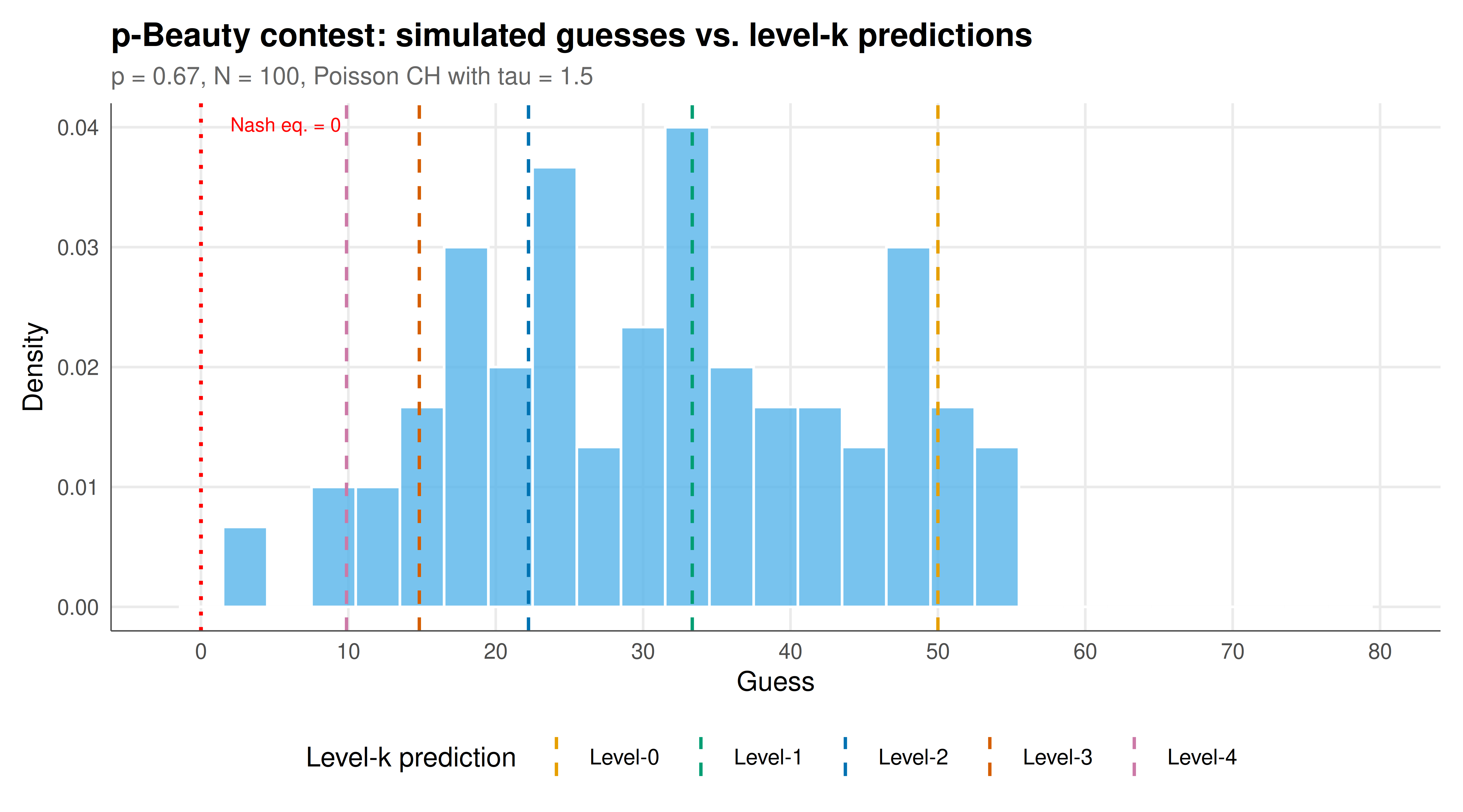
The figure shows a histogram of simulated first-round choices overlaid with the theoretical level-k predictions, demonstrating how level-k thinking generates the characteristic clustering pattern observed in experiments.
```{r}
#| label: fig-beauty-contest-static
#| fig-cap: "Figure 1. Distribution of guesses in a simulated p-beauty contest (p = 2/3, N = 100) with a Poisson CH population (tau = 1.5). Dashed vertical lines mark the pure level-k predictions. The Nash equilibrium at 0 attracts almost no guesses; instead choices cluster around level-1 and level-2 anchors."
#| dev: [png, pdf]
#| fig-width: 9
#| fig-height: 5
#| dpi: 300
# Level-k reference lines
level_lines <- data.frame(
  level = paste0("Level-", 0:4),
  x = sapply(0:4, function(k) level_k_action(k, p))
)

p_static <- ggplot(game, aes(x = choice)) +
  geom_histogram(aes(y = after_stat(density)), binwidth = 3,
                 fill = okabe_ito[2], colour = "white", alpha = 0.8) +
  geom_vline(data = level_lines, aes(xintercept = x, colour = level),
             linetype = "dashed", linewidth = 0.7) +
  geom_vline(xintercept = 0, colour = "red", linetype = "dotted", linewidth = 0.8) +
  annotate("text", x = 2, y = Inf, label = "Nash eq. = 0",
           hjust = 0, vjust = 2, size = 3, colour = "red") +
  scale_colour_manual(values = okabe_ito[c(1, 3, 5, 6, 7)], name = "Level-k prediction") +
  scale_x_continuous(breaks = seq(0, 100, 10), limits = c(-2, 80)) +
  labs(
    title = "p-Beauty contest: simulated guesses vs. level-k predictions",
    subtitle = sprintf("p = %.2f, N = %d, Poisson CH with tau = %.1f", p, N, tau),
    x = "Guess", y = "Density"
  ) +
  theme_publication()

p_static
```
## Interactive figure
The interactive figure tracks the convergence of the mean guess across multiple rounds, showing how repeated play drives behaviour toward the Nash equilibrium.
```{r}
#| label: fig-beauty-contest-interactive
# Prepare data for multi-round visualisation
rounds_plot <- rounds_data %>%
  mutate(
    text = sprintf("Round: %d\nGuess: %.1f", round, choice)
  )

round_means_plot <- round_means %>%
  mutate(
    text = sprintf("Round: %d\nMean guess: %.2f\nTarget: %.2f",
                   round, mean_choice, p * mean_choice)
  )

p_rounds <- ggplot() +
  geom_jitter(data = rounds_plot,
              aes(x = round, y = choice, text = text),
              alpha = 0.15, width = 0.2, colour = okabe_ito[8], size = 0.8) +
  geom_line(data = round_means_plot,
            aes(x = round, y = mean_choice, text = text),
            colour = okabe_ito[5], linewidth = 1.2) +
  geom_point(data = round_means_plot,
             aes(x = round, y = mean_choice, text = text),
             colour = okabe_ito[5], size = 3) +
  geom_hline(yintercept = 0, linetype = "dashed", colour = "red", linewidth = 0.5) +
  scale_x_continuous(breaks = 1:10) +
  labs(
    title = "Convergence of guesses over repeated rounds",
    x = "Round", y = "Guess"
  ) +
  theme_publication()

ggplotly(p_rounds, tooltip = "text") %>%
  config(displaylogo = FALSE)
```
## Interpretation
The simulation results reproduce the key qualitative patterns observed in experimental beauty contest studies. In the first-round data, guesses cluster around the level-1 prediction ($50p \approx 33.3$) and the level-2 prediction ($50p^2 \approx 22.2$) rather than at the Nash equilibrium of 0. This is precisely what Nagel [-@nagel_1995] documented in her seminal experimental study, and what has been replicated across dozens of subsequent experiments with different populations. The level-0 "random" types generate a spread of guesses across the upper range, while the higher-level types produce the distinctive peaks at $50p^k$ that are the signature of iterative best-response reasoning.
The Cognitive Hierarchy model with $\tau \approx 1.5$ provides a good fit to the typical experimental data, implying that the average participant engages in roughly 1.5 steps of strategic reasoning. This estimate is remarkably consistent across studies. The Poisson distribution generates a declining proportion of each successive level: many level-0 and level-1 players, fewer level-2 players, and very few level-3 or higher players. This distribution captures an important empirical regularity: most people do not reason to the Nash equilibrium, but they are not entirely naive either. The majority engage in one or two rounds of "I think that you think that..." reasoning before settling on a choice. The CH model's advantage over the simpler level-k model is that each type best-responds to the correct mixture of lower types rather than assuming everyone else is exactly one level below, which produces more realistic aggregate predictions.
The multi-round convergence dynamics reveal another fundamental insight: learning matters. When the beauty contest is repeated with the same group of players and the mean is announced after each round, guesses converge toward zero, but the convergence is not instantaneous. In our simulation, the mean guess drops from roughly 33 in round 1 to single digits by round 10. The speed of convergence depends on the value of $p$ (lower $p$ values produce faster convergence because the target contracts more quickly) and on the heterogeneity of the population. Importantly, the convergence is not driven by players suddenly discovering the Nash equilibrium through deep reasoning. Instead, it is driven by adaptive learning: players observe the previous round's outcome and adjust their guesses downward, a process more consistent with reinforcement learning or experience-weighted attraction models than with the sudden onset of rational insight.
The gap between Nash equilibrium predictions and observed behaviour in the beauty contest has deep implications for economic theory. If people do not arrive at Nash equilibrium even in a game as simple and transparent as the beauty contest, we should be cautious about assuming equilibrium play in more complex economic environments. The beauty contest demonstrates that the common knowledge of rationality required for iterated dominance arguments --- where each player must be rational, must know that others are rational, must know that others know that they are rational, and so on ad infinitum --- breaks down after just a few levels in practice. This has led researchers to explore alternative solution concepts that incorporate bounded rationality, such as level-k models, quantal response equilibrium, and cursed equilibrium.
The beauty contest also connects to broader questions about coordination and expectation formation. In macroeconomics, models of inflation expectations, asset pricing, and monetary policy transmission all involve agents trying to predict what other agents will do. The beauty contest metaphor suggests that these expectations will be characterised by heterogeneous depths of reasoning, sluggish adjustment, and persistent deviations from the rational expectations benchmark. This connection has motivated a growing literature on "global games" and "higher-order beliefs" that takes seriously the computational and informational limitations that real economic agents face.
One limitation of our simulation is that it uses a known level-k structure rather than more general adaptive learning algorithms. In actual experiments, players use a variety of heuristics and strategies that do not always fit neatly into the level-k framework. Some players anchor on round numbers, others imitate the previous winner, and still others use rules of thumb that are difficult to classify. Structural estimation using maximum likelihood or Bayesian methods can help distinguish between competing models of strategic reasoning, but the data requirements are substantial.
## Extensions & related tutorials
- [Quantal response equilibrium](../../behavioral-gt/quantal-response-equilibrium/) --- models noisy best-responses as an alternative to sharp level-k reasoning
- [Level-k and cognitive hierarchy models](../../behavioral-gt/level-k-cognitive-hierarchy/) --- detailed treatment of structural estimation for level-k and CH models
- [Public goods experiment](../../experimental-economics/public-goods-experiment/) --- another classic experiment revealing bounded rationality in strategic settings
- [Trust game and reciprocity](../../experimental-economics/trust-game-reciprocity/) --- experimental game examining social preferences and strategic reasoning
- [Ultimatum game and fairness](../../behavioral-gt/ultimatum-game-fairness/) --- the role of fairness norms in overriding game-theoretic predictions
## References
::: {#refs}
:::