---
title: "Backward induction and the centipede game paradox"
description: "Implement backward induction for the centipede game in R, demonstrate the dramatic gap between theory and observed play, and analyse how finite vs infinite horizons shape rational behaviour."
author: "Raban Heller"
date: 2026-05-08
date-modified: 2026-05-08
categories:
- foundations
- backward-induction
- centipede-game
- paradox
keywords: ["backward induction", "centipede game", "Rosenthal", "subgame perfection", "rationality paradox"]
labels: ["equilibrium-concepts", "rationality"]
tier: 1
bibliography: ../../../references.bib
vgwort: "TODO_VGWORT_foundations_backward-induction-centipede"
image: thumbnail.png
image-alt: "Centipede game tree with backward induction solution vs observed continuation rates"
citation:
type: webpage
url: https://r-heller.github.io/equilibria/tutorials/foundations/backward-induction-centipede/
license: "CC BY-SA 4.0"
draft: false
has_static_fig: true
has_interactive_fig: true
has_shiny_app: false
---
```{r}
#| label: setup
#| include: false
library(ggplot2)
library(dplyr)
library(tidyr)
library(plotly)
okabe_ito <- c("#E69F00", "#56B4E9", "#009E73", "#F0E442",
"#0072B2", "#D55E00", "#CC79A7", "#999999")
theme_publication <- function(base_size = 12) {
theme_minimal(base_size = base_size) +
theme(plot.title = element_text(size = base_size * 1.2, face = "bold"),
plot.subtitle = element_text(size = base_size * 0.9, color = "grey40"),
axis.line = element_line(color = "grey30", linewidth = 0.3),
panel.grid.minor = element_blank(), legend.position = "bottom",
plot.margin = margin(10, 10, 10, 10))
}
```
## Introduction & motivation
The **centipede game**, introduced by Robert Rosenthal in 1981, is the sharpest illustration of the tension between backward induction and intuitive play. Two players alternate in a sequential game with $K$ stages. At each stage, the active player can either **Take** (ending the game and claiming a larger share of a growing pot) or **Pass** (doubling the pot but giving the opponent the next move). The pot grows exponentially — passing creates enormous potential gains — but backward induction yields a stark prediction: the first player should Take immediately at stage 1, ending the game at its smallest possible pot. The logic is simple but devastating: at the last stage, the active player will Take (since there's no future). Knowing this, the player at stage $K-1$ should Take (since passing leads to being exploited). Unravelling this logic to the beginning gives immediate Take. Yet in every experiment ever run, most players Pass for several rounds, and final-round Take rates are well below 100%. The gap between theory and behaviour is not small — it's categorical. The game thus serves as a litmus test for the limits of common knowledge of rationality: backward induction requires not just that each player is rational, but that each player knows the other is rational, knows that the other knows, and so on — to arbitrary depth. Even a tiny probability that the opponent is "irrational" (willing to cooperate) can justify passing for many rounds, as shown by the reputation models of Kreps, Milgrom, Roberts, and Wilson. This tutorial implements the centipede game for arbitrary length, demonstrates backward induction, simulates play with heterogeneous rationality, and visualises the dramatic gap between theory and observation.
## Mathematical formulation
**Centipede game** with $K$ stages: Pot starts at $(a, b) = (1, 0)$. At stage $k$, if the active player Passes, the pot multiplies; if they Take, payoffs are allocated.
Standard version: at stage $k$, if Take, the taker gets $2^{k-1} + 1$ and the other gets $2^{k-1} - 1$. If the game reaches stage $K$ and the player Passes, payoffs are $(2^{K-1}, 2^K)$.
**Backward induction**: At stage $K$: Take gives $2^{K-1} + 1 > 2^{K-1}$, so Take. At stage $K-1$: knowing opponent Takes at $K$, Take gives more than getting $2^{K-1} - 1$ at $K$. Unravelling: Take at stage 1.
**With bounded rationality**: If player $i$ believes opponent is a "cooperator" (always Passes) with probability $\epsilon > 0$, then passing at early stages has positive expected value even for a fully rational player — the $\epsilon$ chance of continued cooperation outweighs the small immediate gain from Taking.
## R implementation
```{r}
#| label: centipede-game
# === Centipede game with K stages ===
centipede_payoffs <- function(K) {
  # Returns payoff pairs (taker, other) at each stage
  payoffs <- matrix(0, nrow = K, ncol = 2)
  for (k in 1:K) {
    taker_payoff <- 2^(k-1) + 1
    other_payoff <- 2^(k-1) - 1
    payoffs[k, ] <- c(taker_payoff, other_payoff)
  }
  # Final pass payoffs (if both pass all K rounds)
  final_pass <- c(2^(K-1), 2^K)
  list(take_payoffs = payoffs, final_pass = final_pass)
}

K <- 6
game <- centipede_payoffs(K)

cat("=== Centipede Game (K =", K, "stages) ===\n\n")
cat("--- Payoffs at each stage (Taker, Other) ---\n")
for (k in 1:K) {
  player <- ifelse(k %% 2 == 1, "P1", "P2")
  cat(sprintf("  Stage %d (%s moves): Take → (%d, %d)\n",
              k, player, game$take_payoffs[k, 1], game$take_payoffs[k, 2]))
}
cat(sprintf(" Both pass all: (%d, %d)\n", game$final_pass[1], game$final_pass[2]))
cat("\n--- Backward Induction Solution ---\n")
cat(" Result: Player 1 Takes at stage 1\n")
cat(sprintf(" BI payoffs: (%d, %d)\n", game$take_payoffs[1, 1], game$take_payoffs[1, 2]))
cat(sprintf(" Cooperative payoffs: (%d, %d)\n", game$final_pass[1], game$final_pass[2]))
cat(sprintf("  Efficiency loss: %.0f%% of maximum surplus destroyed\n",
            100 * (1 - sum(game$take_payoffs[1, ]) / sum(game$final_pass))))
# === Simulate with heterogeneous rationality ===
set.seed(42)
n_pairs <- 5000

simulate_centipede <- function(K, epsilon, n_pairs) {
  # epsilon = probability each player is a "cooperator" (always passes)
  take_stages <- numeric(n_pairs)
  for (g in 1:n_pairs) {
    is_coop <- runif(2) < epsilon  # each player independently
    stage <- 1
    game_over <- FALSE
    while (stage <= K && !game_over) {
      player <- ifelse(stage %% 2 == 1, 1, 2)
      if (is_coop[player]) {
        stage <- stage + 1  # cooperator always passes
      } else {
        # Rational player: pass if expected value of passing > taking
        # Simplified: pass with probability that decreases as stage increases
        pass_prob <- epsilon^(1 / (K - stage + 1))  # heuristic
        if (runif(1) < pass_prob && stage < K) {
          stage <- stage + 1
        } else {
          take_stages[g] <- stage
          game_over <- TRUE
        }
      }
    }
    if (!game_over) take_stages[g] <- K + 1  # both cooperated to end
  }
  take_stages
}

results <- tibble(
  low_coop = simulate_centipede(K, 0.05, n_pairs),
  med_coop = simulate_centipede(K, 0.20, n_pairs),
  high_coop = simulate_centipede(K, 0.50, n_pairs)
)

cat("\n--- Simulation Results (N =", n_pairs, "pairs) ---\n")
for (eps_label in c("low_coop", "med_coop", "high_coop")) {
  eps_val <- c(low_coop = 0.05, med_coop = 0.20, high_coop = 0.50)[eps_label]
  stages <- results[[eps_label]]
  cat(sprintf("  ε = %.2f: mean take stage = %.2f, %% reaching end = %.1f%%\n",
              eps_val, mean(stages), 100 * mean(stages > K)))
}
```
## Static publication-ready figure
```{r}
#| label: fig-centipede-continuation
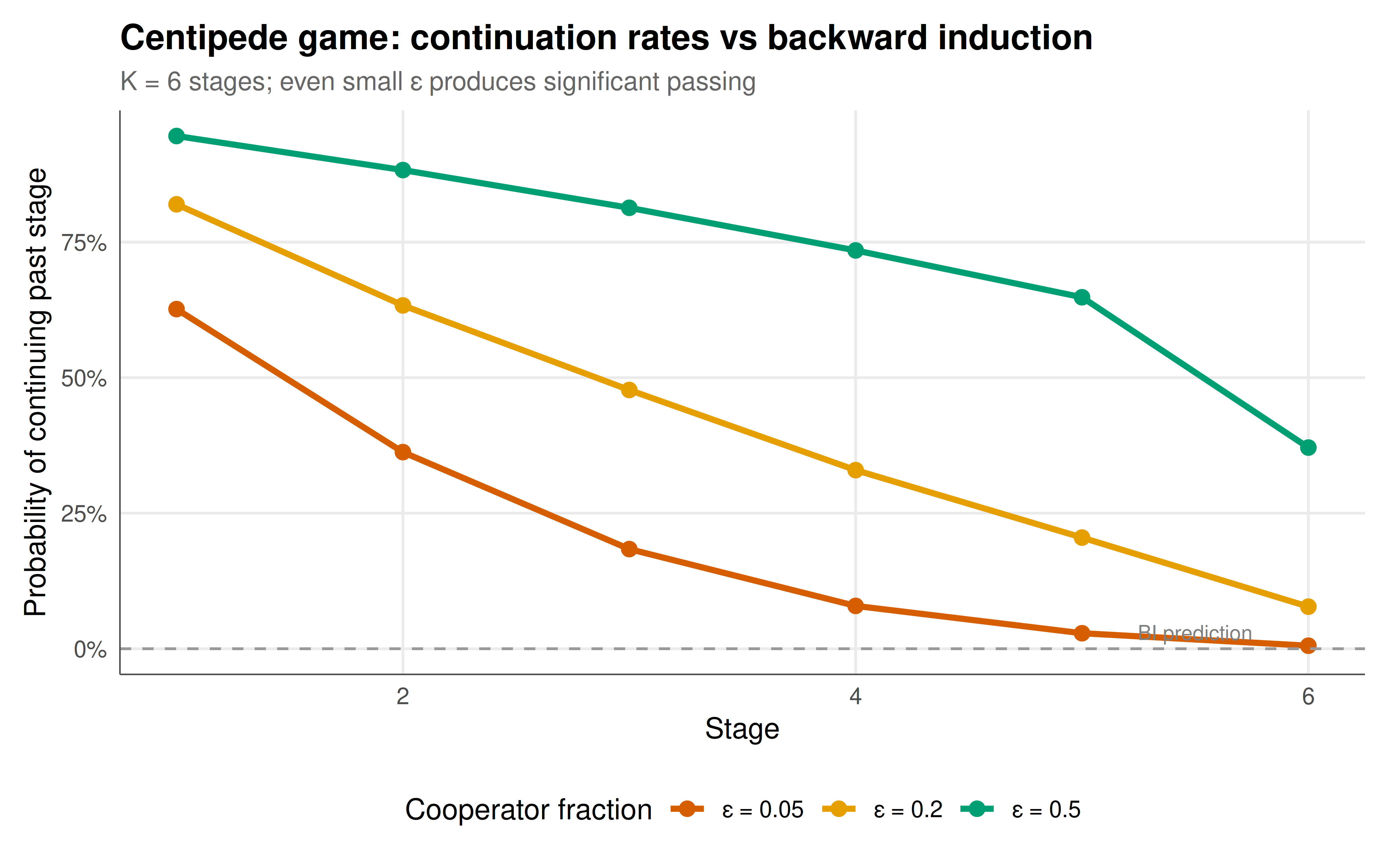
#| fig-cap: "Figure 1. Continuation rates in the centipede game by stage, for different levels of cooperative types (ε). Backward induction predicts 0% continuation at every stage (dashed line). With even a small fraction of cooperators (ε = 5%), play extends significantly beyond stage 1. Higher ε produces continuation patterns matching experimental data — most pairs pass for several rounds before taking. Okabe-Ito palette."
#| dev: [png, pdf]
#| fig-width: 8
#| fig-height: 5
#| dpi: 300
cont_data <- lapply(c(0.05, 0.20, 0.50), function(eps) {
  stages <- simulate_centipede(K, eps, n_pairs)
  sapply(1:K, function(k) mean(stages > k)) |>
    (\(rates) tibble(stage = 1:K, continuation_rate = rates,
                     epsilon = paste0("ε = ", eps)))()
}) |> bind_rows()

ggplot(cont_data, aes(x = stage, y = continuation_rate, color = epsilon)) +
  geom_line(linewidth = 1.2) +
  geom_point(size = 2.5) +
  geom_hline(yintercept = 0, linetype = "dashed", color = "grey60") +
  annotate("text", x = K - 0.5, y = 0.03, label = "BI prediction", color = "grey50", size = 3) +
  scale_color_manual(values = okabe_ito[c(6, 1, 3)], name = "Cooperator fraction") +
  scale_y_continuous(labels = scales::percent_format()) +
  labs(title = "Centipede game: continuation rates vs backward induction",
       subtitle = sprintf("K = %d stages; even small ε produces significant passing", K),
       x = "Stage", y = "Probability of continuing past stage") +
  theme_publication()
```
## Interactive figure
```{r}
#| label: fig-centipede-payoffs
# Show the exponential growth of potential payoffs vs BI outcome
payoff_df <- tibble(
  stage = 0:K,
  total_surplus = c(1, sapply(1:K, function(k) sum(centipede_payoffs(K)$take_payoffs[k, ]))),
  bi_surplus = c(sum(centipede_payoffs(K)$take_payoffs[1, ]), rep(NA, K))
) |>
  pivot_longer(c(total_surplus, bi_surplus), names_to = "type", values_to = "surplus") |>
  filter(!is.na(surplus)) |>
  mutate(
    label = ifelse(type == "total_surplus", "Surplus if Take at stage", "BI outcome"),
    text = paste0("Stage ", stage, "\nTotal surplus: ", surplus, "\nType: ", label)
  )

# Add final cooperation surplus
final_surplus <- tibble(
  stage = K, surplus = sum(centipede_payoffs(K)$final_pass),
  type = "total_surplus", label = "Full cooperation",
  text = paste0("Full cooperation\nTotal surplus: ", sum(centipede_payoffs(K)$final_pass))
)

all_payoffs <- bind_rows(
  payoff_df |> filter(type == "total_surplus"),
  final_surplus
) |> mutate(text = paste0("Stage ", stage, "\nSurplus: ", surplus))

p_payoffs <- ggplot(all_payoffs, aes(x = stage, y = surplus, text = text)) +
  geom_col(fill = okabe_ito[5], alpha = 0.7) +
  geom_hline(yintercept = sum(centipede_payoffs(K)$take_payoffs[1, ]),
             linetype = "dashed", color = okabe_ito[6], linewidth = 1) +
  annotate("text", x = 0.5, y = sum(centipede_payoffs(K)$take_payoffs[1, ]) + 5,
           label = "BI outcome", color = okabe_ito[6], size = 3) +
  labs(title = "Centipede game: exponential surplus growth vs backward induction",
       subtitle = "BI destroys almost all available surplus by stopping at stage 1",
       x = "Stage of Take", y = "Total surplus") +
  theme_publication()

ggplotly(p_payoffs, tooltip = "text") |>
  config(displaylogo = FALSE, modeBarButtonsToRemove = c("select2d", "lasso2d"))
```
## Interpretation
The centipede game crystallises the deepest puzzle in game theory: the assumption of common knowledge of rationality leads to predictions that virtually no human follows. Backward induction is logically airtight — given the premises — but the premises require not just rationality but mutual knowledge of rationality to arbitrary depth. The game shows that even infinitesimal doubt about the opponent's rationality justifies substantial deviation from the BI prediction: with $\epsilon = 5\%$ cooperators, the average game extends well beyond stage 1, and with $\epsilon = 20\%$, play looks similar to experimental data (McKelvey & Palfrey 1992). This connects to the broader literature on reputation effects: Kreps et al. (1982) showed that incomplete information about types can sustain cooperation in finitely repeated games, and the centipede game is the purest example. The exponential surplus growth makes the stakes dramatic — BI leaves almost all surplus on the table. In a 6-stage game, mutual cooperation yields a surplus of 96, while BI yields only 2 — a 98% efficiency loss. This is not a market failure or externality — it is rationality itself that destroys surplus, because the logic of backward induction cannot accommodate the massive gains from mutual trust. The game has deep implications for institutional design: mechanisms that limit the ability to Take (commitment devices), that allow punishment of defection (repeated interaction), or that screen for cooperative types (signaling) can unlock the enormous cooperative surplus that backward induction forecloses. The centipede game remains one of the strongest arguments for bounded rationality and behavioural game theory as complements to classical theory.
## Extensions & related tutorials
- [Extensive-form games and subgame perfection](../extensive-form-subgame-perfection/) — the framework for backward induction.
- [Folk theorem with perfect monitoring](../folk-theorem-perfect-monitoring/) — cooperation in infinitely repeated games.
- [Ultimatum game and fairness](../../behavioral-gt/ultimatum-game-fairness/) — another BI prediction that fails experimentally.
- [Level-k thinking and cognitive hierarchy](../../behavioral-gt/level-k-cognitive-hierarchy/) — bounded rationality models.
- [Trust game and reciprocity](../../experimental-economics/trust-game-reciprocity/) — another cooperation puzzle.
## References
::: {#refs}
:::