---
title: "Cheap talk and strategic communication"
description: "The Crawford-Sobel (1982) cheap talk model: how costless, non-verifiable messages can transmit information when preferences are misaligned, with partition equilibria, information loss as a function of bias, and connections to costly signalling games."
author: "Raban Heller"
date: 2026-05-08
date-modified: 2026-05-08
categories:
- information-theory
- cheap-talk
- strategic-communication
- signalling
keywords: ["cheap talk", "Crawford Sobel", "strategic communication", "partition equilibrium", "information transmission", "sender receiver", "bias", "signalling games", "mutual information"]
labels: ["information-theory", "cheap-talk"]
tier: 1
bibliography: ../../../references.bib
vgwort: "TODO_VGWORT_information-theory_cheap-talk-communication"
image: thumbnail.png
image-alt: "Line plot showing the number of equilibrium partitions and mutual information between sender and receiver as a function of sender bias in the Crawford-Sobel cheap talk model"
citation:
type: webpage
url: https://r-heller.github.io/equilibria/tutorials/information-theory/cheap-talk-communication/
license: "CC BY-SA 4.0"
draft: false
has_static_fig: true
has_interactive_fig: true
has_shiny_app: false
---
```{r}
#| label: setup
#| include: false
library(ggplot2)
library(dplyr)
library(tidyr)
library(plotly)
okabe_ito <- c("#E69F00", "#56B4E9", "#009E73", "#F0E442",
"#0072B2", "#D55E00", "#CC79A7", "#999999")
theme_publication <- function(base_size = 12) {
theme_minimal(base_size = base_size) +
theme(plot.title = element_text(size = base_size * 1.2, face = "bold"),
plot.subtitle = element_text(size = base_size * 0.9, color = "grey40"),
axis.line = element_line(color = "grey30", linewidth = 0.3),
panel.grid.minor = element_blank(), legend.position = "bottom",
plot.margin = margin(10, 10, 10, 10))
}
```
## Introduction & motivation
Communication is one of the most fundamental activities in strategic interaction. Before negotiations, before contracts are signed, before alliances are formed, agents communicate: they share information, make claims, issue warnings, and express preferences. But when agents have conflicting interests, communication becomes strategic. A financial adviser may recommend a product because it is genuinely best for the client, or because it generates the highest commission. A job candidate may describe their qualifications truthfully, or exaggerate their experience. A politician may accurately describe the state of the economy, or spin the data to support their preferred policy. The central question of strategic communication theory is: **how much information can be transmitted through costless, non-verifiable messages when the sender and receiver have different preferences?**
The seminal answer was provided by Crawford and Sobel (1982) in their celebrated cheap talk model. "Cheap talk" refers to communication that is costless to send, non-verifiable (the receiver cannot confirm whether the message is truthful), and non-binding (it does not commit the sender to any action). Under these conditions, one might expect that talk is entirely uninformative --- if lying is free and undetectable, why would a rational receiver pay any attention to the sender's message? Crawford and Sobel showed, remarkably, that cheap talk can transmit information in equilibrium, but the amount of information transmitted is limited by the degree of preference misalignment between sender and receiver.
The model works as follows. A Sender observes a state of the world $\theta$, drawn uniformly from $[0, 1]$. The Sender then sends a costless message $m$ to a Receiver, who takes an action $a$ after observing the message. Both players' payoffs depend on the action and the true state, but they disagree about the ideal action. The Receiver wants $a = \theta$ (match the action to the state), while the Sender wants $a = \theta + b$, where $b > 0$ is the **bias parameter** representing the systematic misalignment in preferences. For example, a financial adviser (Sender) with positive bias always wants the client (Receiver) to invest more than the objectively optimal amount.
Crawford and Sobel proved that the equilibria of this game take the form of **partition equilibria**. The Sender does not reveal the exact state; instead, the Sender divides the state space $[0, 1]$ into a finite number of intervals (partitions) and sends the same message for all states within each interval. The Receiver, upon observing a message, knows only which interval the state belongs to and takes the optimal action given that interval (the midpoint, under uniform prior). The number of partitions in the most informative equilibrium is determined by the bias: when bias is small, many partitions are possible, and communication is relatively informative. As bias increases, fewer partitions can be sustained in equilibrium, and information transmission degrades. When bias is very large, only the **babbling equilibrium** (one partition, no information) is sustainable.
This result provides a precise characterisation of the "limits of talk." It explains why communication between parties with aligned interests is rich and informative (small bias, many partitions), while communication between adversaries is coarse and uninformative (large bias, few partitions). The model has been applied to understand expert advice, legislative communication, diplomatic signalling, and organisational communication, among many other settings.
In this tutorial, we derive and implement the Crawford-Sobel partition equilibria for different bias levels, compute the equilibrium partition structure, and measure information transmission using mutual information. We show how the number of sustainable partitions decreases with bias, how the partition intervals become increasingly unequal, and how the total information transmitted (in bits) degrades as preferences diverge. We then connect cheap talk to costly signalling games, where the key difference --- signals have direct costs --- enables full information revelation even with misaligned preferences.
## Mathematical formulation
**Setup.** The state $\theta \sim U[0, 1]$. The Sender observes $\theta$ and sends message $m$. The Receiver observes $m$ and chooses action $a$. Payoffs are:
$$
U_S(a, \theta) = -(a - \theta - b)^2, \quad U_R(a, \theta) = -(a - \theta)^2
$$
where $b > 0$ is the Sender's bias. Both players dislike deviations from their ideal, but the Sender's ideal action exceeds the Receiver's by $b$.
**Partition equilibrium.** An $N$-partition equilibrium is defined by cutpoints $0 = t_0 < t_1 < \cdots < t_N = 1$ such that:
1. **Receiver optimality**: upon receiving a message indicating $\theta \in [t_{k-1}, t_k]$, the Receiver chooses $a_k = (t_{k-1} + t_k)/2$ (the conditional expectation).
2. **Sender indifference at boundaries**: the Sender at state $\theta = t_k$ is indifferent between reporting the $k$-th and $(k+1)$-th interval:
$$
-(a_k - t_k - b)^2 = -(a_{k+1} - t_k - b)^2
$$
This yields the **indifference condition**:
$$
a_k + a_{k+1} = 2(t_k + b)
$$
Substituting $a_k = (t_{k-1} + t_k)/2$ and $a_{k+1} = (t_k + t_{k+1})/2$:
$$
t_{k+1} = 2t_k - t_{k-1} + 4b
$$
This is a second-order linear recurrence. Starting from $t_0 = 0$, given $t_1$, we can compute all subsequent cutpoints. The value of $t_1$ is determined by the boundary condition $t_N = 1$.
**Maximum number of partitions.** An $N$-partition equilibrium exists if and only if:
$$
N(N-1) \cdot 2b < 1 \quad \Longleftrightarrow \quad N < \frac{1}{2}\left(1 + \sqrt{1 + \frac{2}{b}}\right)
$$
**Mutual information.** The mutual information between state $\theta$ and action $a$ (in nats) measures the information transmitted:
$$
I(\theta; a) = H(\theta) - H(\theta | a) = \log(1) - \sum_{k=1}^N \frac{t_k - t_{k-1}}{1} \cdot \log(t_k - t_{k-1})
$$
where $H(\theta) = 0$ (entropy of $U[0,1]$ in the differential sense; we use the discrete partition entropy for comparison):
$$
I_N = -\sum_{k=1}^N (t_k - t_{k-1}) \log_2(t_k - t_{k-1})
$$
which is maximised at $\log_2(N)$ when all intervals are equal.
## R implementation
We compute the Crawford-Sobel partition equilibria for a range of bias values and measure information transmission.
```{r}
#| label: cheap-talk-simulation
# --- Compute CS partition equilibrium ---
# Given bias b and number of partitions N, solve for cutpoints
compute_cs_partition <- function(b, N) {
  if (N == 1) return(list(cutpoints = c(0, 1), valid = TRUE))

  # Use the recurrence: t_{k+1} = 2*t_k - t_{k-1} + 4b
  # with t_0 = 0, and find t_1 such that t_N = 1
  # Analytical solution: t_k = k*t_1 + k*(k-1)*2b
  # Setting t_N = 1: N*t_1 + N*(N-1)*2b = 1
  # => t_1 = (1 - 2*N*(N-1)*b) / N

  t1 <- (1 - 2 * N * (N - 1) * b) / N

  if (t1 <= 0) return(list(cutpoints = NULL, valid = FALSE))

  cutpoints <- numeric(N + 1)
  cutpoints[1] <- 0
  cutpoints[2] <- t1

  for (k in 2:N) {
    cutpoints[k + 1] <- 2 * cutpoints[k] - cutpoints[k - 1] + 4 * b
  }

  # Check validity: all cutpoints increasing and t_N = 1
  valid <- all(diff(cutpoints) > 1e-10) & abs(cutpoints[N + 1] - 1) < 1e-6
  list(cutpoints = cutpoints, valid = valid)
}

# --- Maximum partitions for given bias ---
max_partitions <- function(b) {
  floor(0.5 * (1 + sqrt(1 + 2/b)))
}

# --- Mutual information of a partition ---
mutual_info <- function(cutpoints) {
  widths <- diff(cutpoints)
  widths <- widths[widths > 0]
  -sum(widths * log2(widths))
}

# --- Expected loss for Receiver ---
receiver_loss <- function(cutpoints) {
  widths <- diff(cutpoints)
  # E[(theta - a_k)^2 | theta in interval k] = width_k^2 / 12
  sum(widths * widths^2 / 12)
}

# --- Compute for range of biases ---
bias_values <- seq(0.005, 0.25, by = 0.005)

results <- tibble()

for (b in bias_values) {
  N_max <- max_partitions(b)
  for (N in 1:N_max) {
    cs <- compute_cs_partition(b, N)
    if (cs$valid) {
      mi <- mutual_info(cs$cutpoints)
      rl <- receiver_loss(cs$cutpoints)
      widths <- diff(cs$cutpoints)
      results <- bind_rows(results, tibble(
        bias = b, N = N, N_max = N_max,
        mutual_info = mi,
        receiver_loss = rl,
        max_width = max(widths),
        min_width = min(widths),
        width_ratio = max(widths) / min(widths)
      ))
    }
  }
}

# Focus on the most informative equilibrium for each bias
most_informative <- results %>%
  group_by(bias) %>%
  filter(N == max(N)) %>%
  ungroup()

# --- Summary ---
cat("=== Cheap Talk: Crawford-Sobel Partition Equilibria ===\n\n")
cat(" --- Maximum partitions by bias ---\n")
cat(sprintf("  %-8s | %-6s | %-12s | %-14s | %-12s\n",
            "Bias (b)", "N_max", "Mut. info", "Receiver loss", "Width ratio"))
cat(paste(rep("-", 68), collapse = ""), "\n")
key_biases <- c(0.01, 0.02, 0.05, 0.1, 0.15, 0.2, 0.25)
for (b in key_biases) {
  row <- most_informative %>% filter(abs(bias - b) < 0.001)
  if (nrow(row) > 0) {
    cat(sprintf("  %-8.3f | %6d | %12.3f | %14.4f | %12.2f\n",
                row$bias, row$N, row$mutual_info, row$receiver_loss,
                row$width_ratio))
  }
}
# --- Example: partition structure for b = 0.05 ---
b_example <- 0.05
N_example <- max_partitions(b_example)
cs_example <- compute_cs_partition(b_example, N_example)

cat(sprintf("\n  --- Example partition: b = %.2f, N = %d ---\n", b_example, N_example))
cat(sprintf("  Cutpoints: %s\n",
            paste(round(cs_example$cutpoints, 4), collapse = ", ")))
cat(sprintf("  Interval widths: %s\n",
            paste(round(diff(cs_example$cutpoints), 4), collapse = ", ")))
cat(sprintf("  Actions (midpoints): %s\n",
            paste(round((cs_example$cutpoints[-length(cs_example$cutpoints)] +
                         cs_example$cutpoints[-1]) / 2, 4), collapse = ", ")))
# --- Simulate actual communication for a specific bias ---
set.seed(42)
n_sim <- 10000
b_sim <- 0.05
N_sim <- max_partitions(b_sim)
cs_sim <- compute_cs_partition(b_sim, N_sim)

theta_sim <- runif(n_sim)
# Determine which partition each theta falls in
partition_sim <- findInterval(theta_sim, cs_sim$cutpoints, rightmost.closed = TRUE)
partition_sim <- pmin(partition_sim, N_sim)
# Receiver's action = midpoint of the partition
action_sim <- (cs_sim$cutpoints[partition_sim] + cs_sim$cutpoints[partition_sim + 1]) / 2

# Compare with babbling (N=1) and full revelation
action_babble <- rep(0.5, n_sim)
action_full   <- theta_sim

loss_cs     <- mean((action_sim - theta_sim)^2)
loss_babble <- mean((action_babble - theta_sim)^2)
loss_full   <- 0

cat(sprintf("\n  --- Simulated communication (b = %.2f, N = %d, n = %d) ---\n",
            b_sim, N_sim, n_sim))
cat(sprintf(" Receiver's expected loss (CS equilibrium): %.4f\n", loss_cs))
cat(sprintf(" Receiver's expected loss (babbling): %.4f\n", loss_babble))
cat(sprintf(" Receiver's expected loss (full revelation): %.4f\n", loss_full))
cat(sprintf("  Information improvement over babbling:      %.1f%%\n",
            (1 - loss_cs / loss_babble) * 100))
# --- Prepare simulation data for plotting ---
sim_df <- tibble(
  theta = theta_sim,
  action = action_sim,
  partition = factor(partition_sim)
) %>%
  sample_n(min(2000, n_sim))  # subsample for plotting
```
## Static publication-ready figure
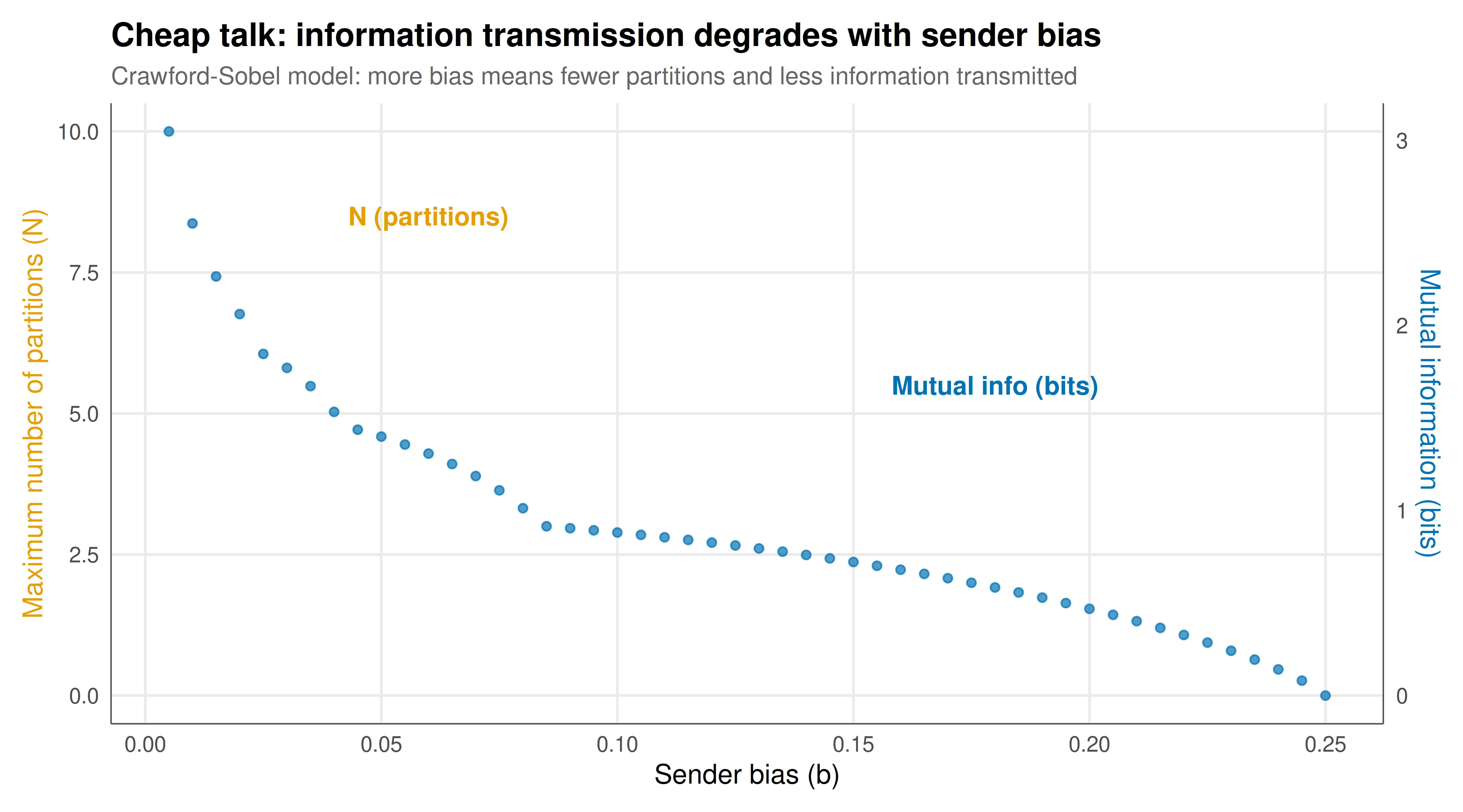
The figure shows how the maximum number of equilibrium partitions and the mutual information between state and action decline as sender bias increases, illustrating the fundamental trade-off between preference alignment and information transmission.
```{r}
#| label: fig-cheap-talk-static
#| fig-cap: "Figure 1. Information transmission in the Crawford-Sobel cheap talk model as a function of sender bias. Left axis (orange): maximum number of equilibrium partitions (step function). Right axis (blue): mutual information in bits for the most informative equilibrium. As bias increases, fewer partitions are sustainable and less information is transmitted, converging to the babbling equilibrium (N = 1, I = 0 bits) for large bias."
#| dev: [png, pdf]
#| fig-width: 9
#| fig-height: 5
#| dpi: 300
# Combine N_max and mutual info on dual axis
scale_factor <- max(most_informative$N) / max(most_informative$mutual_info)

p_cheaptalk <- ggplot(most_informative) +
  geom_step(aes(x = bias, y = N,
                text = paste0("Bias: ", bias,
                              "\nMax partitions: ", N,
                              "\nMutual info: ", round(mutual_info, 3), " bits")),
            color = okabe_ito[1], linewidth = 1.2) +
  geom_line(aes(x = bias, y = mutual_info * scale_factor,
                text = paste0("Bias: ", bias,
                              "\nMutual info: ", round(mutual_info, 3), " bits",
                              "\nMax partitions: ", N)),
            color = okabe_ito[5], linewidth = 1.2) +
  geom_point(aes(x = bias, y = mutual_info * scale_factor),
             color = okabe_ito[5], size = 1.5, alpha = 0.7) +
  scale_y_continuous(
    name = "Maximum number of partitions (N)",
    sec.axis = sec_axis(~ . / scale_factor, name = "Mutual information (bits)")
  ) +
  labs(
    title = "Cheap talk: information transmission degrades with sender bias",
    subtitle = "Crawford-Sobel model: more bias means fewer partitions and less information transmitted",
    x = "Sender bias (b)"
  ) +
  annotate("text", x = 0.06, y = max(most_informative$N) * 0.85,
           label = "N (partitions)", color = okabe_ito[1],
           size = 4, fontface = "bold") +
  annotate("text", x = 0.18, y = max(most_informative$N) * 0.55,
           label = "Mutual info (bits)", color = okabe_ito[5],
           size = 4, fontface = "bold") +
  theme_publication() +
  theme(
    axis.title.y.left = element_text(color = okabe_ito[1]),
    axis.title.y.right = element_text(color = okabe_ito[5])
  )

p_cheaptalk
```
## Interactive figure
Explore how equilibrium partitions and information transmission change with bias. Hover over points to see the exact number of partitions and bits of information for each bias level.
```{r}
#| label: fig-cheap-talk-interactive
# For plotly, use a single-axis version focused on mutual information
p_mi <- ggplot(most_informative,
               aes(x = bias, y = mutual_info,
                   text = paste0("Bias: ", bias,
                                 "\nMax partitions: ", N,
                                 "\nMutual information: ", round(mutual_info, 3), " bits",
                                 "\nReceiver loss: ", round(receiver_loss, 4),
                                 "\nWidth ratio (max/min): ", round(width_ratio, 1)))) +
  geom_line(color = okabe_ito[5], linewidth = 1) +
  geom_point(aes(color = factor(N)), size = 3, alpha = 0.8) +
  scale_color_manual(
    values = okabe_ito[1:length(unique(most_informative$N))],
    name = "N (partitions)"
  ) +
  labs(
    title = "Information transmission in cheap talk equilibria",
    subtitle = "Mutual information (bits) vs sender bias, coloured by number of partitions",
    x = "Sender bias (b)",
    y = "Mutual information (bits)"
  ) +
  theme_publication() +
  theme(legend.position = "bottom")

ggplotly(p_mi, tooltip = "text") %>%
  config(displaylogo = FALSE) %>%
  layout(legend = list(orientation = "h", y = -0.2))
```
## Interpretation
The Crawford-Sobel model reveals a precise and elegant relationship between preference alignment and the possibility of informative communication. The results demonstrate several key insights.
**Communication is possible even with misaligned preferences**, but it is coarse. Even when the Sender has a positive bias and thus always wants to induce a higher action than is optimal for the Receiver, equilibria exist in which the Sender's message conveys some information about the state. The Sender cannot lie arbitrarily, because the Receiver rationally interprets messages knowing the Sender's incentives. In equilibrium, the Sender reveals the "neighbourhood" of the true state (which partition it falls in) but not its exact value.
**More bias means less communication.** The maximum number of sustainable partitions decreases sharply with the bias parameter $b$. At $b = 0.01$ (nearly aligned preferences), up to 8 partitions are possible, transmitting almost 3 bits of information --- the Receiver learns which octile of the state space the true state lies in. At $b = 0.1$, only 3 partitions are possible, and less than 1.5 bits are transmitted. At $b = 0.25$, only the babbling equilibrium (one partition, zero information) survives. The relationship is governed by the condition $N < \frac{1}{2}(1 + \sqrt{1 + 2/b})$, which provides an exact characterisation of the "limits of talk."
**Partition intervals are unequal.** In the most informative equilibrium, the intervals are not equally spaced. They grow wider as $\theta$ increases, because the recurrence $t_{k+1} = 2t_k - t_{k-1} + 4b$ causes each successive interval to be $4b$ wider than the previous one. This asymmetry means that the Sender communicates more precisely about low states than high states. Intuitively, the Sender's upward bias creates more temptation to exaggerate at higher states, so the equilibrium must allow coarser messages there to maintain credibility.
**The welfare implications are nuanced.** Compared to babbling, the most informative equilibrium substantially reduces the Receiver's expected loss. But compared to full revelation (which is not achievable in cheap talk with $b > 0$), substantial information is lost. The percentage improvement over babbling provides a useful metric: at moderate bias levels, cheap talk recovers 60-80 percent of the information that full revelation would provide, which is a remarkable achievement for a costless communication protocol.
The connection to **costly signalling** is instructive. In Spence's (1973) job market signalling model and its descendants, the key difference is that signals have direct costs (e.g., the cost of education). These costs can separate types: if high-ability workers find education less costly, they can credibly signal their type by acquiring more education. In cheap talk, there are no such costs, so separation must be achieved through the equilibrium structure (partitions) rather than through differential costs. This is why cheap talk produces only partial separation (intervals) while costly signalling can produce full separation (each type sends a distinct signal). The choice between cheap talk and costly signalling depends on whether the available communication channels have inherent costs --- a question that is central to institutional design in organisations, markets, and politics.
## Extensions & related tutorials
- [Entropy and strategic information](../../information-theory/entropy-and-strategic-information/) --- information-theoretic foundations for measuring information in strategic settings
- [Value of information in games](../../information-theory/value-of-information-games/) --- how the ability to acquire information before acting changes strategic outcomes
- [Bayesian games with incomplete information](../../bayesian-methods/bayesian-games-incomplete-information/) --- the formal framework for games where players have private information
- [Mechanism design](../../mechanism-design/) --- designing institutions that incentivise truthful communication (the "revelation principle")
- [Global games and coordination](../../bayesian-methods/global-games-coordination/) --- how information structure (public vs private signals) affects coordination outcomes
## References
::: {#refs}
:::