---
title: "Introduction to mechanism design — engineering incentives in strategic environments"
description: "Survey the foundations of mechanism design as 'reverse game theory,' covering the revelation principle, Gibbard-Satterthwaite impossibility, and implementation theory, with a worked R implementation of the pivotal mechanism for public goods provision."
author: "Raban Heller"
date: 2026-05-08
date-modified: 2026-05-08
categories:
- mechanism-design
- revelation-principle
- gibbard-satterthwaite
- implementation-theory
keywords: ["mechanism design", "revelation principle", "Gibbard-Satterthwaite", "incentive compatibility", "pivotal mechanism", "public goods", "social choice"]
labels: ["mechanism-design", "foundations"]
tier: 1
bibliography: ../../../references.bib
vgwort: "TODO_VGWORT_mechanism-design_mechanism-design-intro"
image: thumbnail.png
image-alt: "Diagram showing the relationship between social choice functions, mechanisms, and the revelation principle"
citation:
type: webpage
url: https://r-heller.github.io/equilibria/tutorials/mechanism-design/mechanism-design-intro/
license: "CC BY-SA 4.0"
draft: false
has_static_fig: true
has_interactive_fig: true
has_shiny_app: false
---
```{r}
#| label: setup
#| include: false
library(ggplot2)
library(dplyr)
library(tidyr)
library(plotly)
okabe_ito <- c("#E69F00", "#56B4E9", "#009E73", "#F0E442",
"#0072B2", "#D55E00", "#CC79A7", "#999999")
theme_publication <- function(base_size = 12) {
theme_minimal(base_size = base_size) +
theme(
plot.title = element_text(size = base_size * 1.2, face = "bold"),
plot.subtitle = element_text(size = base_size * 0.9, color = "grey40"),
axis.line = element_line(color = "grey30", linewidth = 0.3),
panel.grid.minor = element_blank(),
legend.position = "bottom",
plot.margin = margin(10, 10, 10, 10)
)
}
```
## Introduction & motivation
Game theory traditionally takes the rules of a game as given and asks: how will rational agents behave? **Mechanism design** inverts this question: given the behaviour we desire, what rules should we design? This "reverse game theory" perspective transforms economics from a purely analytical discipline into an engineering one, where the designer crafts institutions, auctions, voting rules, or contracts that channel self-interested behaviour toward socially desirable outcomes.
The intellectual foundations were laid by Leonid Hurwicz, who in 1960 formalised the notion of a **mechanism** as a communication system — a set of messages that agents can send, together with an outcome function that maps message profiles to social decisions [@hurwicz_1960]. Hurwicz asked the fundamental question: can we design mechanisms that implement desirable social outcomes even when agents have private information and act strategically? The answer, as we shall see, is nuanced: some goals are achievable and others are provably impossible, and the boundary between the two is delineated by celebrated impossibility theorems.
Two results form the theoretical backbone of the field. The **revelation principle** (Gibbard 1973, Myerson 1979) states that for any mechanism that implements a social choice function in some equilibrium, there exists a **direct** mechanism — one where agents simply report their private information — that implements the same function truthfully. This enormously simplifies mechanism design: rather than searching over the infinite space of possible mechanisms (sealed-bid auctions, ascending auctions, multi-round negotiations, etc.), the designer need only consider direct revelation mechanisms where truth-telling is an equilibrium. The **Gibbard-Satterthwaite theorem** (1973, 1975) establishes a fundamental impossibility: any deterministic social choice function defined over three or more alternatives that is strategy-proof (truthful reporting is a dominant strategy for every agent) and onto (every alternative can be selected) must be **dictatorial** — one agent's preferences entirely determine the outcome [@gibbard_1973]. This impossibility result, the strategic counterpart of Arrow's impossibility theorem, means that no voting system can simultaneously be non-dictatorial, strategy-proof, and unrestricted over three or more candidates.
These results together define the design space: the revelation principle tells us where to look (direct mechanisms), and the Gibbard-Satterthwaite theorem tells us what we cannot find (non-dictatorial strategy-proof rules over unrestricted domains). The genius of mechanism design lies in escaping impossibility by restricting the domain (e.g., quasi-linear preferences), relaxing the solution concept (e.g., Bayesian rather than dominant-strategy implementation), or accepting weaker desiderata (e.g., efficiency without budget balance). The VCG mechanism, the most important positive result in the field, achieves efficiency and dominant-strategy incentive compatibility in quasi-linear environments by sacrificing budget balance — it may run a surplus or deficit. This tutorial provides the conceptual foundations, implements a pivotal mechanism for public goods, and illustrates the impossibility results computationally.
## Mathematical formulation
**Environment**: A set of agents $N = \{1, \ldots, n\}$, a set of alternatives $A$, and a type space $\Theta_i$ for each agent. Agent $i$'s type $\theta_i \in \Theta_i$ represents their private information (preferences, valuations).
**Social choice function**: A mapping $f: \Theta_1 \times \cdots \times \Theta_n \to A$ specifying the desired outcome for each type profile.
**Mechanism**: A pair $(\mathcal{M}, g)$ where $\mathcal{M} = \mathcal{M}_1 \times \cdots \times \mathcal{M}_n$ is the message space and $g: \mathcal{M} \to A$ is the outcome function.
**Implementation**: Mechanism $(\mathcal{M}, g)$ implements $f$ in dominant strategies if there exists a strategy profile $s^* = (s_1^*, \ldots, s_n^*)$ such that:
$$
g(s_i^*(\theta_i), m_{-i}) \succeq_{\theta_i} g(m_i', m_{-i}) \quad \forall \theta_i, \forall m_i', \forall m_{-i}
$$
and $g(s^*(\theta)) = f(\theta)$ for all type profiles $\theta$.
**Revelation principle**: If mechanism $(\mathcal{M}, g)$ implements $f$ via strategy profile $s^*$, then the **direct** mechanism $(\Theta, f)$ — where agents report types and the outcome function is $f$ itself — implements $f$ truthfully: $s_i^*(\theta_i) = \theta_i$.
**Gibbard-Satterthwaite theorem**: If $|A| \geq 3$ and $f: \mathcal{L}(A)^n \to A$ is surjective and strategy-proof (where $\mathcal{L}(A)$ is the set of strict linear orders over $A$), then $f$ is dictatorial.
**Pivotal (Clarke) mechanism** for public goods: $n$ agents with quasi-linear utilities $u_i = \theta_i k - t_i$, where $k \in \{0, 1\}$ is the public good decision and $t_i$ is a monetary transfer. The mechanism:
1. Collects reports $\hat{\theta}_i$
2. Provides the good if $\sum_i \hat{\theta}_i \geq C$ (where $C$ is the cost)
3. Charges pivotal agents: $t_i = C - \sum_{j \neq i} \hat{\theta}_j$ if agent $i$ is pivotal (their report changes the decision), else $t_i = 0$
## R implementation
```{r}
#| label: pivotal-mechanism
set.seed(42)

# Pivotal mechanism for binary public good provision
pivotal_mechanism <- function(valuations, cost) {
  n <- length(valuations)
  total_value <- sum(valuations)
  provide <- total_value >= cost

  payments <- numeric(n)
  is_pivotal <- logical(n)

  for (i in 1:n) {
    others_total <- sum(valuations[-i])
    # Would decision change without agent i?
    provide_without_i <- others_total >= cost

    if (provide != provide_without_i) {
      is_pivotal[i] <- TRUE
      if (provide) {
        # Agent i caused provision: pay the gap
        payments[i] <- cost - others_total
      } else {
        # Agent i caused non-provision: compensate others
        payments[i] <- -(others_total - cost)
      }
    }
  }

  utilities <- ifelse(provide, valuations, 0) - payments

  list(
    provide = provide,
    payments = payments,
    utilities = utilities,
    is_pivotal = is_pivotal,
    total_value = total_value,
    cost = cost,
    surplus = total_value - cost
  )
}

# Example: 8 agents, public good costs 50
n_agents <- 8
cost <- 50
valuations <- c(15, 12, 8, 7, 5, 4, 3, 2)

result <- pivotal_mechanism(valuations, cost)

cat("Public good provision (pivotal mechanism):\n")
cat(sprintf(" Cost of public good: %d\n", cost))
cat(sprintf(" Total reported valuation: %d\n", result$total_value))
cat(sprintf(" Decision: %s\n", ifelse(result$provide, "PROVIDE", "DO NOT PROVIDE")))
cat("\nAgent details:\n")
cat(" Agent | Valuation | Pivotal | Payment | Utility\n")
cat(" ------|-----------|---------|---------|--------\n")
for (i in 1:n_agents) {
  cat(sprintf("  %5d | %9d | %7s | %7.1f | %7.1f\n",
              i, valuations[i],
              ifelse(result$is_pivotal[i], "YES", "no"),
              result$payments[i], result$utilities[i]))
}
cat(sprintf("\n Total payments collected: %.1f\n", sum(result$payments)))
cat(sprintf("  Budget surplus/deficit: %.1f\n",
            sum(result$payments) - ifelse(result$provide, cost, 0)))
```
```{r}
#| label: incentive-compatibility-verification
# Verify DSIC: no agent benefits from misreporting
cat("--- Incentive compatibility check ---\n\n")
for (agent in 1:3) {
  truthful_utility <- result$utilities[agent]
  best_deviation_utility <- truthful_utility
  best_deviation_report <- valuations[agent]

  # Test a range of misreports
  test_reports <- seq(0, 30, by = 0.5)
  for (fake_val in test_reports) {
    fake_valuations <- valuations
    fake_valuations[agent] <- fake_val
    fake_result <- pivotal_mechanism(fake_valuations, cost)
    # Agent's TRUE utility under fake mechanism outcome
    true_utility_under_fake <- ifelse(fake_result$provide, valuations[agent], 0) - fake_result$payments[agent]
    if (true_utility_under_fake > best_deviation_utility + 1e-10) {
      best_deviation_utility <- true_utility_under_fake
      best_deviation_report <- fake_val
    }
  }

  cat(sprintf("Agent %d (true val = %d): truthful utility = %.1f, best deviation utility = %.1f\n",
              agent, valuations[agent], truthful_utility, best_deviation_utility))
  cat(sprintf("  -> Truthful reporting is optimal: %s\n\n",
              ifelse(abs(best_deviation_utility - truthful_utility) < 1e-10, "YES", "NO")))
}
```
```{r}
#| label: impossibility-demonstration
# Demonstrate Gibbard-Satterthwaite: explore strategy-proofness of common voting rules
set.seed(42)

# Plurality voting: each voter votes for top choice
# Borda count: each voter assigns n-1 points to top, n-2 to second, etc.
# Check if these are strategy-proof

alternatives <- c("A", "B", "C")

# Generate preference profiles (each row = voter's ranking)
# 3 voters, 3 alternatives
prefs <- list(
  c("A", "B", "C"),
  c("B", "C", "A"),
  c("C", "A", "B")
)

# Plurality rule
plurality_winner <- function(prefs) {
  top_choices <- sapply(prefs, function(p) p[1])
  tab <- table(top_choices)
  names(which.max(tab))
}

# Borda count
borda_winner <- function(prefs) {
  n_alt <- length(prefs[[1]])
  scores <- setNames(numeric(n_alt), prefs[[1]])
  scores[] <- 0
  for (p in prefs) {
    for (k in 1:n_alt) {
      scores[p[k]] <- scores[p[k]] + (n_alt - k)
    }
  }
  names(which.max(scores))
}

cat("Gibbard-Satterthwaite impossibility demonstration:\n\n")
# Check manipulability of plurality
cat("Plurality voting:\n")
true_winner_plur <- plurality_winner(prefs)
cat(sprintf("  True preferences -> Winner: %s\n", true_winner_plur))
# Voter 2 (prefers B > C > A) tries strategic voting
manipulated <- FALSE
for (perm_idx in 1:6) {
  all_perms <- list(
    c("A", "B", "C"), c("A", "C", "B"), c("B", "A", "C"),
    c("B", "C", "A"), c("C", "A", "B"), c("C", "B", "A")
  )
  fake_prefs <- prefs
  fake_prefs[[2]] <- all_perms[[perm_idx]]
  new_winner <- plurality_winner(fake_prefs)
  # Voter 2's true ranking: B > C > A
  true_rank_old <- which(prefs[[2]] == true_winner_plur)
  true_rank_new <- which(prefs[[2]] == new_winner)
  if (true_rank_new < true_rank_old) {
    cat(sprintf("  Voter 2 reports %s -> Winner: %s (improvement from rank %d to %d)\n",
                paste(fake_prefs[[2]], collapse = ">"), new_winner,
                true_rank_old, true_rank_new))
    manipulated <- TRUE
    break
  }
}
if (!manipulated) cat("  No beneficial manipulation found for voter 2\n")

# Check manipulability of Borda
cat("\nBorda count:\n")
true_winner_borda <- borda_winner(prefs)
cat(sprintf("  True preferences -> Winner: %s\n", true_winner_borda))
manipulated_borda <- FALSE
for (voter in 1:3) {
  for (perm_idx in 1:6) {
    all_perms <- list(
      c("A", "B", "C"), c("A", "C", "B"), c("B", "A", "C"),
      c("B", "C", "A"), c("C", "A", "B"), c("C", "B", "A")
    )
    fake_prefs <- prefs
    fake_prefs[[voter]] <- all_perms[[perm_idx]]
    new_winner <- borda_winner(fake_prefs)
    true_rank_old <- which(prefs[[voter]] == true_winner_borda)
    true_rank_new <- which(prefs[[voter]] == new_winner)
    if (true_rank_new < true_rank_old) {
      cat(sprintf("  Voter %d reports %s -> Winner: %s (rank %d to %d)\n",
                  voter, paste(fake_prefs[[voter]], collapse = ">"),
                  new_winner, true_rank_old, true_rank_new))
      manipulated_borda <- TRUE
      break
    }
  }
  if (manipulated_borda) break
}
if (!manipulated_borda) cat("  No beneficial manipulation found\n")

cat("\nConclusion: Both plurality and Borda are manipulable, consistent with\n")
cat("the Gibbard-Satterthwaite theorem (no non-dictatorial surjective SCF\n")
cat("over 3+ alternatives is strategy-proof).\n")
```
```{r}
#| label: simulation-pivotal-properties
# Simulate pivotal mechanism across many random problems
set.seed(42)
n_sims <- 1000
n_agents_sim <- 10
cost_sim <- 30

sim_results <- data.frame()

for (s in 1:n_sims) {
  vals <- runif(n_agents_sim, min = 0, max = 10)
  res <- pivotal_mechanism(vals, cost_sim)

  sim_results <- rbind(sim_results, data.frame(
    sim = s,
    total_value = res$total_value,
    provided = res$provide,
    total_payment = sum(res$payments),
    n_pivotal = sum(res$is_pivotal),
    budget_surplus = sum(res$payments) - ifelse(res$provide, cost_sim, 0),
    efficient = (res$provide == (res$total_value >= cost_sim))
  ))
}

cat("Pivotal mechanism simulation (1000 random problems, 10 agents, cost = 30):\n")
cat(sprintf(" Provision rate: %.1f%%\n", 100 * mean(sim_results$provided)))
cat(sprintf(" Efficiency rate: %.1f%%\n", 100 * mean(sim_results$efficient)))
cat(sprintf(" Avg pivotal agents: %.2f\n", mean(sim_results$n_pivotal)))
cat(sprintf("  Avg budget surplus (when provided): %.2f\n",
            mean(sim_results$budget_surplus[sim_results$provided])))
cat(sprintf("  Budget deficit cases: %d\n",
            sum(sim_results$budget_surplus < -0.01)))
```
## Static publication-ready figure
```{r}
#| label: fig-mechanism-properties
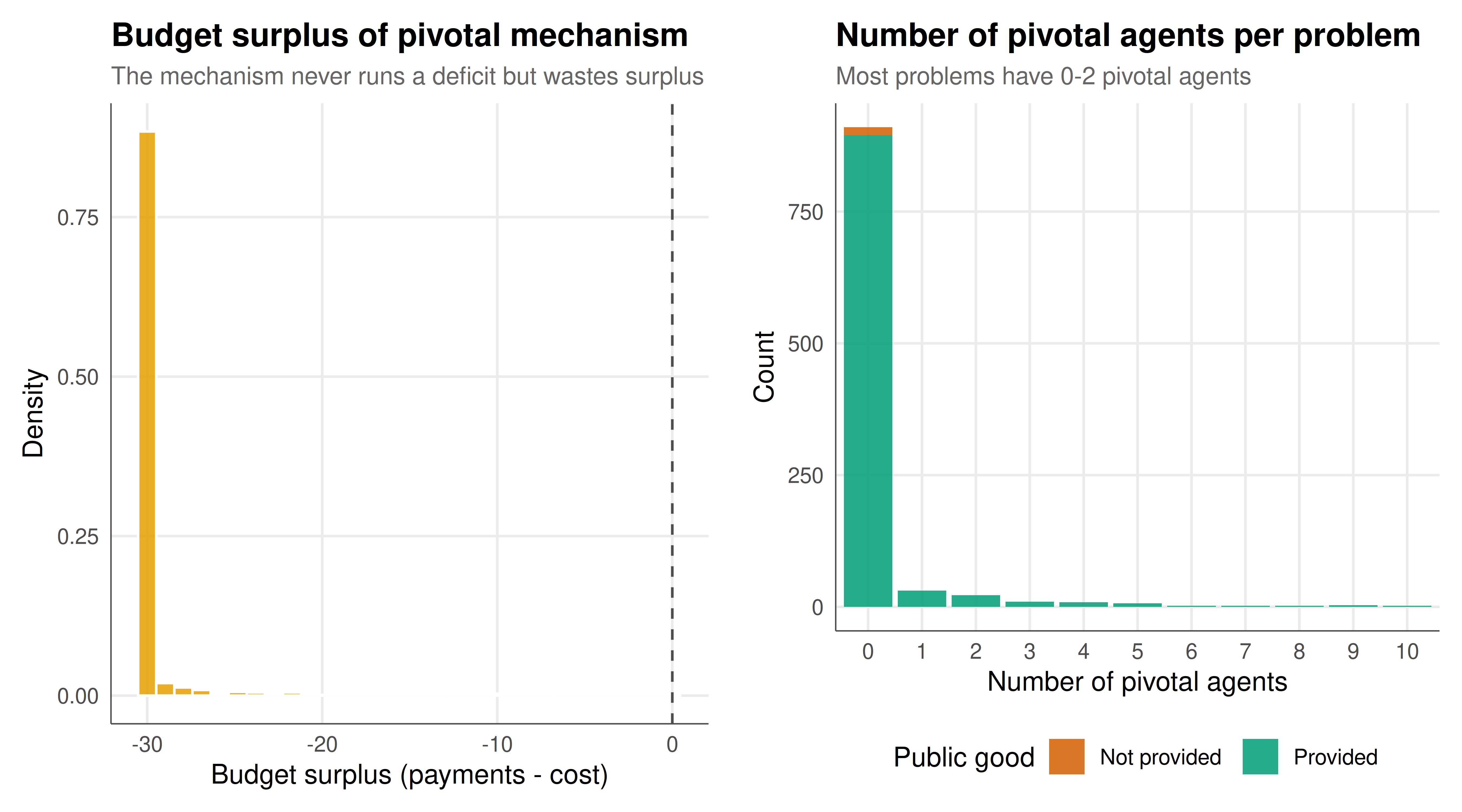
#| fig-cap: "Properties of the pivotal mechanism across 1000 random public goods problems: budget surplus and number of pivotal agents"
#| fig-width: 9
#| fig-height: 5
#| dev: [png, pdf]
#| dpi: 300
provided_df <- sim_results %>% filter(provided)

p1 <- ggplot(provided_df, aes(x = budget_surplus)) +
  geom_histogram(aes(y = after_stat(density)), bins = 30,
                 fill = okabe_ito[1], color = "white", alpha = 0.85) +
  geom_vline(xintercept = 0, linetype = "dashed", color = "grey30") +
  labs(
    title = "Budget surplus of pivotal mechanism",
    subtitle = "The mechanism never runs a deficit but wastes surplus",
    x = "Budget surplus (payments - cost)", y = "Density"
  ) +
  theme_publication()

p2 <- ggplot(sim_results, aes(x = factor(n_pivotal), fill = provided)) +
  geom_bar(position = "stack", alpha = 0.85) +
  scale_fill_manual(values = c("TRUE" = okabe_ito[3], "FALSE" = okabe_ito[6]),
                    labels = c("TRUE" = "Provided", "FALSE" = "Not provided")) +
  labs(
    title = "Number of pivotal agents per problem",
    subtitle = "Most problems have 0-2 pivotal agents",
    x = "Number of pivotal agents", y = "Count",
    fill = "Public good"
  ) +
  theme_publication()

# Combine using patchwork-style approach with gridExtra
gridExtra::grid.arrange(p1, p2, ncol = 2)
```
## Interactive figure
```{r}
#| label: fig-mechanism-interactive
#| fig-cap: "Interactive exploration of pivotal mechanism properties (hover for simulation details)"
interactive_df <- sim_results %>%
  filter(provided) %>%
  mutate(tooltip_text = paste0(
    "Simulation: ", sim, "\n",
    "Total value: ", round(total_value, 1), "\n",
    "Total payment: ", round(total_payment, 1), "\n",
    "Budget surplus: ", round(budget_surplus, 1), "\n",
    "Pivotal agents: ", n_pivotal
  ))

p_interactive <- ggplot(interactive_df,
                        aes(x = total_value, y = total_payment,
                            color = factor(n_pivotal),
                            text = tooltip_text)) +
  geom_point(alpha = 0.6, size = 1.5) +
  geom_abline(intercept = 0, slope = 1, linetype = "dashed", color = "grey50") +
  scale_color_manual(values = okabe_ito[1:6]) +
  labs(
    title = "Payments vs. total value in pivotal mechanism",
    x = "Total agent valuations", y = "Total payments collected",
    color = "Pivotal agents"
  ) +
  theme_publication()

ggplotly(p_interactive, tooltip = "text") %>%
  config(displaylogo = FALSE)
```
## Interpretation
The pivotal mechanism illustrates both the power and the limitations of mechanism design. On the positive side, the mechanism achieves two remarkable properties simultaneously: **allocative efficiency** (the public good is provided if and only if total value exceeds cost, which is the socially optimal decision) and **dominant-strategy incentive compatibility** (every agent's best strategy is to report their true valuation, regardless of what others do). The incentive compatibility check confirms that no agent can improve their utility by misreporting — the mechanism aligns individual incentives with social optimality.
However, the mechanism violates **budget balance**: the payments collected from pivotal agents generally do not equal the cost of the public good. The simulations show that the pivotal mechanism always runs a weakly positive budget surplus (never a deficit), but this surplus is "wasted" — it cannot be redistributed to agents without destroying incentive compatibility. This is a manifestation of the **Green-Laffont impossibility theorem**: no mechanism can simultaneously achieve efficiency, incentive compatibility, and budget balance in the public goods setting.
The Gibbard-Satterthwaite demonstration reveals the fundamental tension in social choice: both plurality voting and Borda count — the two most widely used voting rules — are susceptible to strategic manipulation. A voter can sometimes improve their outcome by misrepresenting their preferences. The theorem tells us this is not a design flaw specific to these rules; it is an inherent limitation of any non-dictatorial voting system over three or more alternatives. This impossibility is what makes mechanism design both necessary (we must work within these constraints) and challenging (we must find creative ways to circumvent or weaken the impossibility conditions).
The contrast between the impossibility in general social choice and the possibility in quasi-linear environments (where agents have monetary transfers available) is one of the deepest insights in the field: money "lubricates" incentive design by providing a flexible transfer instrument that can compensate agents for truthful behaviour.
## Extensions & related tutorials
- **[VCG mechanism](../vcg-mechanism/)**: The general efficient mechanism for quasi-linear environments, of which the pivotal mechanism is a special case.
- **[Vickrey second-price auction](../vickrey-second-price-auction/)**: The single-item auction that launched mechanism design, demonstrating DSIC in the simplest possible setting.
- **[Deferred acceptance](../deferred-acceptance/)**: Strategy-proof matching mechanisms that operate outside the quasi-linear framework.
- **[Voting power indices](../../cooperative-gt/voting-power-indices/)**: Weighted voting games where power and weight diverge, connecting to the impossibility of fair social choice.
- **[Public goods game with punishment](../../behavioral-gt/public-goods-punishment/)**: How behavioural mechanisms (punishment) can sustain cooperation where standard mechanisms require monetary transfers.
## References
::: {#refs}
:::