---
title: "Centrality measures for game-theoretic network analysis"
description: "Compute degree, betweenness, and eigenvector centrality for strategic networks using igraph in R, and visualise how different centrality measures reveal distinct power structures in game-theoretic settings."
author: "Raban Heller"
date: 2026-05-08
categories:
- network-science
- centrality
- graph-theory
keywords: ["centrality", "degree centrality", "betweenness centrality", "eigenvector centrality", "igraph", "network analysis", "power structures", "game theory", "R"]
labels: ["network-science", "centrality-analysis"]
tier: 1
bibliography: ../../../references.bib
vgwort: "TODO_VGWORT_network-science_centrality-measures-game-theory"
image: thumbnail.png
image-alt: "Network graph with nodes coloured by eigenvector centrality revealing the power structure of a strategic network"
citation:
type: webpage
url: https://r-heller.github.io/equilibria/tutorials/network-science/centrality-measures-game-theory/
license: "CC BY-SA 4.0"
draft: false
has_static_fig: true
has_interactive_fig: true
---
```{r}
#| label: setup
#| include: false
library(ggplot2)
library(dplyr)
library(tidyr)
library(plotly)
okabe_ito <- c("#E69F00", "#56B4E9", "#009E73", "#F0E442",
"#0072B2", "#D55E00", "#CC79A7", "#999999")
theme_publication <- function(base_size = 12) {
theme_minimal(base_size = base_size) +
theme(
plot.title = element_text(size = base_size * 1.2, face = "bold"),
plot.subtitle = element_text(size = base_size * 0.9, color = "grey40"),
axis.line = element_line(color = "grey30", linewidth = 0.3),
panel.grid.minor = element_blank(),
legend.position = "bottom",
plot.margin = margin(10, 10, 10, 10)
)
}
```
## Introduction & motivation
In strategic networks — alliances between firms, coalitions among legislators, information-sharing agreements between intelligence agencies — not all positions are equal. Some agents occupy structurally advantageous positions that grant them disproportionate influence over outcomes. Centrality measures from network science provide the formal tools to identify and quantify these structural advantages. But which centrality measure is appropriate depends on the strategic context: degree centrality counts direct connections (relevant when influence flows only to neighbours), betweenness centrality measures control over information flow between others (relevant in brokerage and intermediation), and eigenvector centrality accounts for the quality of connections — being connected to well-connected agents matters more than sheer quantity. In game-theoretic networks, these distinctions are not academic: a player with high betweenness can extract rents by serving as a broker; a player with high eigenvector centrality may have outsized influence in coordination games where actions propagate through the network. The Shapley value and Myerson value from cooperative game theory connect directly to centrality — in many network games, a player's Shapley value is proportional to their centrality score. This tutorial computes all three centrality measures for a range of stylised and random networks using igraph, visualises how they disagree on which nodes are "most central," and interprets the differences through a game-theoretic lens. Understanding centrality is prerequisite for network formation models, public goods games on networks, and the growing literature on targeting and seeding in social networks.
## Mathematical formulation
Given an undirected network $g = (V, E)$ with $n$ nodes, we define three centrality measures.
**Degree centrality** counts direct connections, normalised by the maximum possible:
$$
C_D(i) = \frac{d_i}{n - 1}
$$
where $d_i = |\{j : ij \in E\}|$ is the degree of node $i$.
**Betweenness centrality** measures the fraction of shortest paths that pass through node $i$:
$$
C_B(i) = \sum_{s \neq i \neq t} \frac{\sigma_{st}(i)}{\sigma_{st}}
$$
where $\sigma_{st}$ is the total number of shortest paths from $s$ to $t$ and $\sigma_{st}(i)$ is the number passing through $i$. This is normalised by dividing by $(n-1)(n-2)/2$.
**Eigenvector centrality** assigns each node a score proportional to the sum of its neighbours' scores. Formally, $\mathbf{c}_E$ is the eigenvector corresponding to the largest eigenvalue $\lambda_1$ of the adjacency matrix $\mathbf{A}$:
$$
\mathbf{A} \mathbf{c}_E = \lambda_1 \mathbf{c}_E, \quad c_{E,i} \geq 0, \quad \|\mathbf{c}_E\| = 1
$$
By the Perron-Frobenius theorem, for connected graphs, $\lambda_1 > 0$ and $\mathbf{c}_E$ has all positive entries.
## R implementation
We compute all three centrality measures for several network structures and analyse where they agree and disagree.
```{r}
#| label: centrality-implementation
library(igraph)

# Compute centrality measures for a network
compute_centralities <- function(g, name = "Network") {
  tibble(
    node = seq_len(vcount(g)),
    network = name,
    degree = degree(g, normalized = TRUE),
    betweenness = betweenness(g, normalized = TRUE),
    eigenvector = eigen_centrality(g)$vector
  )
}

# --- Create stylised networks ---
n <- 10
set.seed(42)

# Star: one hub connected to all
star <- make_star(n, mode = "undirected")

# Line: path graph
line <- make_graph(edges = unlist(lapply(1:(n-1), function(i) c(i, i+1))),
                   n = n, directed = FALSE)

# Core-periphery: 4-clique core + 6 peripheral nodes each connected to 1 core node
core_periph <- make_full_graph(4, directed = FALSE)
core_periph <- add_vertices(core_periph, 6)
core_periph <- add_edges(core_periph, c(1,5, 2,6, 3,7, 4,8, 1,9, 3,10))

# Barabasi-Albert preferential attachment
ba <- sample_pa(n, m = 2, directed = FALSE)

networks <- list(
  "Star" = star,
  "Line" = line,
  "Core-periphery" = core_periph,
  "Preferential attachment" = ba
)

# Compute centralities for all networks
all_centralities <- bind_rows(lapply(names(networks), function(name) {
  compute_centralities(networks[[name]], name)
}))

# Print summary
cat("=== Centrality comparison across network structures (n=10) ===\n")
summary_stats <- all_centralities |>
  group_by(network) |>
  summarise(
    max_degree_node = node[which.max(degree)],
    max_between_node = node[which.max(betweenness)],
    max_eigen_node = node[which.max(eigenvector)],
    degree_gini = 1 - sum((sort(degree)/sum(degree))^2),
    .groups = "drop"
  )
print(as.data.frame(summary_stats))
# Correlation between measures
cat("\n=== Rank correlations (Spearman) within each network ===\n")
correlations <- all_centralities |>
  group_by(network) |>
  summarise(
    deg_vs_btw = cor(degree, betweenness, method = "spearman"),
    deg_vs_eig = cor(degree, eigenvector, method = "spearman"),
    btw_vs_eig = cor(betweenness, eigenvector, method = "spearman"),
    .groups = "drop"
  )
print(as.data.frame(correlations))
```
## Static publication-ready figure
```{r}
#| label: fig-centrality-static
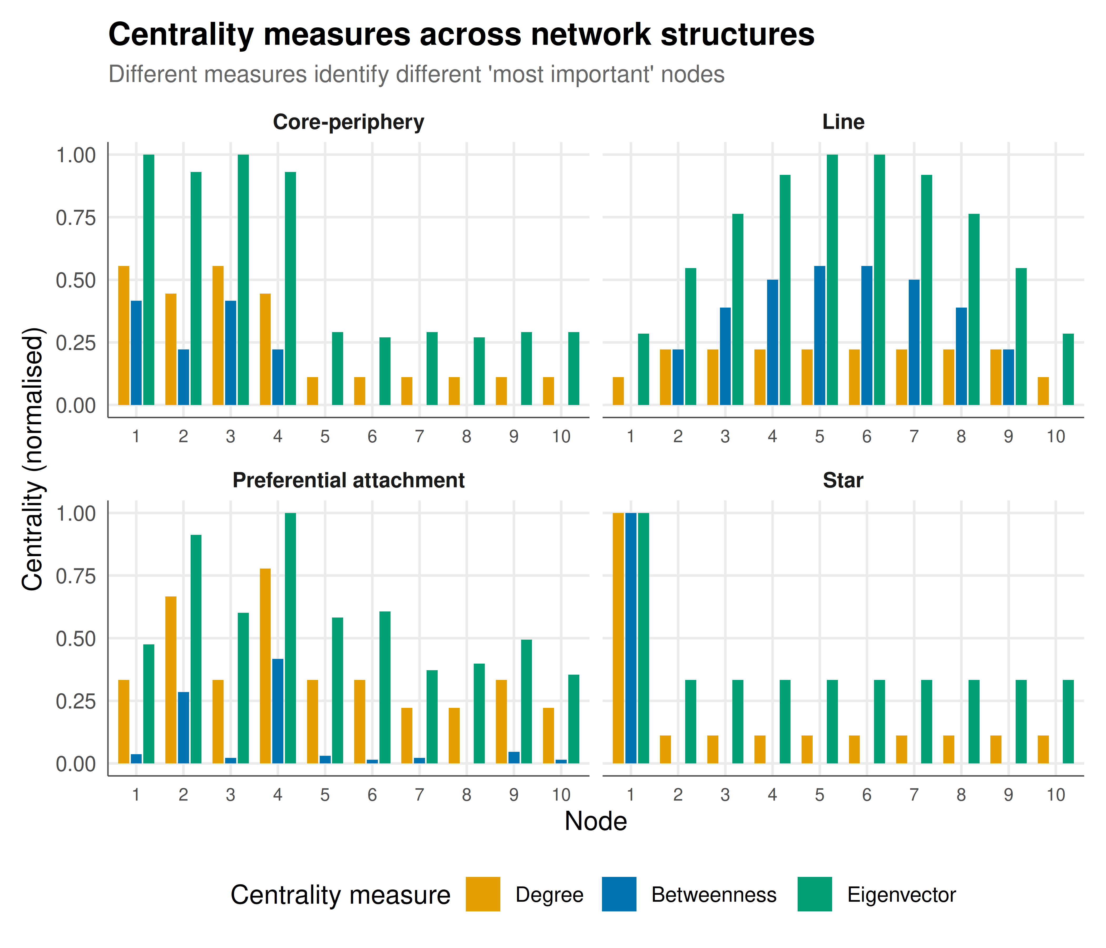
#| fig-cap: "Figure 1. Comparison of degree, betweenness, and eigenvector centrality across four network structures (n = 10). Nodes are ordered by degree centrality within each network. The measures agree in the star network (the hub dominates on all counts) but diverge in the line graph (central nodes have high betweenness but moderate degree) and the core-periphery network (core nodes dominate on eigenvector centrality). Okabe-Ito palette."
#| dev: [png, pdf]
#| fig-width: 7
#| fig-height: 6
#| dpi: 300
centralities_long <- all_centralities |>
  pivot_longer(cols = c(degree, betweenness, eigenvector),
               names_to = "measure",
               values_to = "centrality") |>
  mutate(measure = factor(measure,
    levels = c("degree", "betweenness", "eigenvector"),
    labels = c("Degree", "Betweenness", "Eigenvector")
  ))

# Rank nodes within each network by degree for consistent ordering
centralities_long <- centralities_long |>
  group_by(network) |>
  mutate(node_rank = dense_rank(desc(
    centrality[measure == "Degree"][match(node, node[measure == "Degree"])]
  ))) |>
  ungroup()

p_cent <- ggplot(centralities_long,
                  aes(x = factor(node), y = centrality, fill = measure)) +
  geom_col(position = position_dodge(width = 0.8), width = 0.7) +
  facet_wrap(~network, ncol = 2, scales = "free_x") +
  scale_fill_manual(values = c("Degree" = okabe_ito[1],
                                 "Betweenness" = okabe_ito[5],
                                 "Eigenvector" = okabe_ito[3]),
                     name = "Centrality measure") +
  labs(
    title = "Centrality measures across network structures",
    subtitle = "Different measures identify different 'most important' nodes",
    x = "Node", y = "Centrality (normalised)"
  ) +
  theme_publication() +
  theme(strip.text = element_text(face = "bold"),
        axis.text.x = element_text(size = 8))

p_cent
```
## Interactive figure
```{r}
#| label: fig-centrality-interactive
# Scatter plot: degree vs eigenvector centrality, with betweenness as size
scatter_data <- all_centralities |>
  mutate(text = paste0("Node: ", node,
                       "\nDegree: ", round(degree, 3),
                       "\nBetweenness: ", round(betweenness, 3),
                       "\nEigenvector: ", round(eigenvector, 3)))

p_scatter <- ggplot(scatter_data,
                     aes(x = degree, y = eigenvector,
                         size = betweenness + 0.01,
                         color = network, text = text)) +
  geom_point(alpha = 0.7) +
  geom_abline(slope = 1, intercept = 0, linetype = "dashed", color = "grey50") +
  scale_color_manual(values = c("Star" = okabe_ito[1],
                                  "Line" = okabe_ito[5],
                                  "Core-periphery" = okabe_ito[3],
                                  "Preferential attachment" = okabe_ito[6]),
                      name = "Network") +
  scale_size_continuous(range = c(2, 10), name = "Betweenness") +
  labs(
    title = "Degree vs. eigenvector centrality",
    subtitle = "Point size = betweenness centrality; dashed line = perfect agreement",
    x = "Degree centrality", y = "Eigenvector centrality"
  ) +
  theme_publication()

ggplotly(p_scatter, tooltip = "text") |>
  config(displaylogo = FALSE,
         modeBarButtonsToRemove = c("select2d", "lasso2d"))
```
## Interpretation
The three centrality measures capture fundamentally different notions of structural power, and their disagreements are game-theoretically meaningful. In the star network, all three measures agree: the hub is the most central node by any definition — it has the most connections, controls all shortest paths, and is connected to every other node. This unanimity reflects the unambiguous structural dominance of the hub position. In the line graph, however, the measures diverge sharply. The middle nodes have moderate degree but very high betweenness — they control all traffic between the two halves of the network. This makes them powerful brokers in information-exchange games but not necessarily influential in coordination games. Eigenvector centrality penalises them less than betweenness rewards them, because their neighbours are themselves not highly connected. The core-periphery network reveals the most interesting disagreements. Core nodes have similar degree to each other, but eigenvector centrality differentiates among them based on their connection to other core members. A core node connected to three other core nodes and one peripheral node scores higher on eigenvector centrality than one connected to two core nodes and two peripheral nodes — even though their degrees are identical. This is precisely the distinction that matters in games where influence propagates: being connected to influential agents amplifies your own influence recursively. For game theorists, the choice of centrality measure should be guided by the underlying strategic model: degree for local interactions, betweenness for intermediation and brokerage, and eigenvector for recursive influence and coordination.
## Extensions & related tutorials
- [Strategic network formation — who links with whom?](../../network-games/network-formation-strategic/) — how strategic agents form the networks we analyse.
- [Public goods games on networks](../../network-games/public-goods-networks/) — centrality predicts free-riding and contribution patterns.
- [Matrix games — linear algebra foundations](../../linear-algebra-matrix/matrix-games-and-linear-algebra/) — eigenvector centrality connects to spectral graph theory.
- [Cooperative game theory — Shapley value](../../cooperative-gt/shapley-value/) — the Shapley value as a centrality-like concept.
- [Spatial evolutionary games](../../evolutionary-gt/spatial-games/) — network position affects evolutionary fitness.
## References
::: {#refs}
:::