---
title: "Game Theory Environments for Reinforcement Learning in R"
description: "Build OpenAI Gym-inspired game theory environments in pure R using R6 classes with reset(), step(), and render() methods. Implement Q-learning agents that learn Nash equilibrium strategies in Prisoner's Dilemma and Hawk-Dove games."
author: "Raban Heller"
date: 2026-05-08
date-modified: 2026-05-08
categories:
- public-apis-and-datasets
- reinforcement-learning
- game-environments
keywords: ["reinforcement learning", "Q-learning", "game environment", "R6 classes", "Nash equilibrium convergence"]
labels: ["machine-learning", "simulation"]
tier: 1
bibliography: ../../../references.bib
vgwort: "TODO_VGWORT_public-apis-and-datasets_openai-gym-game-environments"
image: thumbnail.png
image-alt: "Q-learning convergence plot showing agents learning Nash equilibrium strategies in iterated Prisoner's Dilemma and Hawk-Dove games"
citation:
type: webpage
url: https://r-heller.github.io/equilibria/tutorials/public-apis-and-datasets/openai-gym-game-environments/
license: "CC BY-SA 4.0"
draft: false
has_static_fig: true
has_interactive_fig: true
has_shiny_app: false
---
```{r}
#| label: setup
#| include: false
library(ggplot2)
library(dplyr)
library(tidyr)
library(plotly)
okabe_ito <- c("#E69F00", "#56B4E9", "#009E73", "#F0E442",
"#0072B2", "#D55E00", "#CC79A7", "#999999")
theme_publication <- function(base_size = 12) {
theme_minimal(base_size = base_size) +
theme(plot.title = element_text(size = base_size * 1.2, face = "bold"),
plot.subtitle = element_text(size = base_size * 0.9, color = "grey40"),
axis.line = element_line(color = "grey30", linewidth = 0.3),
panel.grid.minor = element_blank(), legend.position = "bottom",
plot.margin = margin(10, 10, 10, 10))
}
```
## Introduction & motivation
Reinforcement learning (RL) has transformed the study of sequential decision-making, producing agents that master complex games from Atari to Go. The OpenAI Gym framework, introduced in 2016, established a standard interface for RL environments: every environment exposes `reset()`, `step()`, and `render()` methods, enabling researchers to develop and test learning algorithms independently of the specific task. While Gym was designed for single-agent settings, the multi-agent extension --- where multiple learning agents interact strategically --- is the natural domain of game theory. The intersection of reinforcement learning and game theory asks a fundamental question: when independent learning agents interact repeatedly in a strategic environment, do their learned strategies converge to a game-theoretic equilibrium?
This tutorial builds a complete game theory environment framework in pure R, using R6 classes to implement the Gym-style interface. R6 classes, unlike R's traditional S3 and S4 systems, use reference semantics (objects are mutable and passed by reference), which is natural for environments that maintain internal state across method calls. Our framework supports any two-player normal-form game played repeatedly, and we demonstrate it on two canonical games: the Prisoner's Dilemma and the Hawk-Dove game. These games represent fundamentally different strategic structures --- the Prisoner's Dilemma has a dominant-strategy equilibrium where both players defect, while the Hawk-Dove game has a unique mixed-strategy equilibrium --- and the learning dynamics in each game are correspondingly different.
The Q-learning agent we implement is the simplest model-free RL algorithm that is guaranteed to converge in single-agent settings with finite state and action spaces. In a multi-agent game-theoretic context, the convergence guarantees of Q-learning are considerably weaker, because the environment is non-stationary from each agent's perspective (the other agent is simultaneously learning and changing its strategy). Nevertheless, empirical studies have shown that Q-learning agents can converge to Nash equilibrium strategies in a variety of games, particularly when the learning rate and exploration rate are decayed appropriately. Our implementation tracks the agents' action probabilities (derived from their Q-values via softmax or epsilon-greedy policies) over the course of training, allowing us to visualize the convergence process and assess how closely the learned strategies approximate the Nash equilibrium.
The Prisoner's Dilemma, first formalized in the 1950s and extensively studied by @axelrod_1984, represents the fundamental tension between individual rationality and collective welfare. Each player can Cooperate (C) or Defect (D), with the payoff structure ensuring that Defect is a dominant strategy (it yields a higher payoff regardless of the opponent's choice), but mutual cooperation yields a higher payoff than mutual defection. In the one-shot game, the unique Nash equilibrium is mutual defection. In the iterated (repeated) game, more complex strategies like Tit-for-Tat can sustain cooperation, but in our memoryless Q-learning framework (where the agent does not condition on history), the agents should converge to the stage-game Nash equilibrium of mutual defection.
The Hawk-Dove game (also known as the Chicken game) models conflict over a shared resource. Each player can play Hawk (aggressive) or Dove (passive). If both play Hawk, they fight and both suffer. If both play Dove, they share the resource equally. If one plays Hawk and the other Dove, the Hawk takes the entire resource. The unique symmetric Nash equilibrium is in mixed strategies: each player plays Hawk with a specific probability that depends on the payoff parameters. This makes the Hawk-Dove game particularly interesting for RL experiments, because the learning agents must converge not to a deterministic action but to a specific mixing probability.
By implementing the entire framework in pure R without any Python dependencies, we ensure that the code is self-contained, reproducible, and accessible to R users who may not have Python or the OpenAI Gym library installed. The R6 class structure provides a clean, extensible interface that can be extended to support more complex game structures (extensive-form games, stochastic games, games with continuous action spaces) and more sophisticated learning algorithms (policy gradient methods, actor-critic architectures, multi-agent variants of deep Q-networks).
## Mathematical formulation
**Stage game.** A two-player normal-form game with action sets $A_1 = A_2 = \{a_1, a_2\}$ and payoff matrices $U_1, U_2 \in \mathbb{R}^{2 \times 2}$.
**Iterated game.** The stage game is played for $T$ rounds. At each round $t$, both players simultaneously choose actions $a_t^1, a_t^2$ and receive payoffs $r_t^i = U_i(a_t^1, a_t^2)$.
**Q-learning update.** For a stateless (memoryless) agent, the Q-value for action $a$ is updated after observing reward $r$:
$$
Q_{t+1}(a) = Q_t(a) + \alpha_t \bigl[r_t - Q_t(a)\bigr]
$$
where $\alpha_t \in (0, 1)$ is the learning rate at time $t$.
**Epsilon-greedy policy.** The agent selects:
$$
a_t = \begin{cases}
\arg\max_a Q_t(a) & \text{with probability } 1 - \varepsilon_t \\
\text{uniform random action} & \text{with probability } \varepsilon_t
\end{cases}
$$
**Boltzmann (softmax) policy.** Alternatively:
$$
\Pr(a_t = a) = \frac{\exp(\beta \cdot Q_t(a))}{\sum_{a'} \exp(\beta \cdot Q_t(a'))}
$$
where $\beta > 0$ is the inverse temperature.
**Nash equilibrium convergence.** We say the agents **converge to Nash** if the empirical action frequencies $\hat{p}_T^i(a) = \frac{1}{T}\sum_{t=1}^T \mathbb{1}[a_t^i = a]$ satisfy:
$$
\lim_{T \to \infty} \hat{p}_T^i \to \sigma_i^*
$$
where $\sigma^* = (\sigma_1^*, \sigma_2^*)$ is a Nash equilibrium of the stage game.
**Game payoff matrices:**
*Prisoner's Dilemma* (NE: both Defect):
$$
U_1 = U_2 = \begin{pmatrix} -1 & -3 \\ 0 & -2 \end{pmatrix}
\quad \text{(rows: C/D, cols: C/D)}
$$
*Hawk-Dove* (NE: mixed, $p^* = \frac{v}{c}$):
$$
U_1 = U_2 = \begin{pmatrix} \frac{v-c}{2} & v \\ 0 & \frac{v}{2} \end{pmatrix}
$$
With $v = 4, c = 6$: $p^*(\text{Hawk}) = v/c = 2/3$.
## R implementation
```{r}
#| label: rl-environments
#| code-fold: false
set.seed(2024)

# ================================================================
# R6 Class: GameEnvironment (Gym-style interface)
# ================================================================

library(R6)

GameEnvironment <- R6Class("GameEnvironment",
  public = list(
    name = NULL,
    actions = NULL,
    payoff1 = NULL,
    payoff2 = NULL,
    n_actions = NULL,
    history = NULL,
    t = 0,

    initialize = function(name, actions, payoff1, payoff2) {
      self$name <- name
      self$actions <- actions
      self$n_actions <- length(actions)
      self$payoff1 <- payoff1
      self$payoff2 <- payoff2
      self$reset()
    },

    reset = function() {
      self$t <- 0
      self$history <- list(actions1 = integer(), actions2 = integer(),
                           rewards1 = numeric(), rewards2 = numeric())
      invisible(list(observation = 0, info = list(game = self$name)))
    },

    step = function(action1, action2) {
      self$t <- self$t + 1
      r1 <- self$payoff1[action1, action2]
      r2 <- self$payoff2[action1, action2]

      self$history$actions1 <- c(self$history$actions1, action1)
      self$history$actions2 <- c(self$history$actions2, action2)
      self$history$rewards1 <- c(self$history$rewards1, r1)
      self$history$rewards2 <- c(self$history$rewards2, r2)

      list(rewards = c(r1, r2), observation = 0,
           done = FALSE, info = list(t = self$t))
    },

    render = function() {
      if (self$t == 0) {
        cat(sprintf("[%s] No actions taken yet.\n", self$name))
        return(invisible(NULL))
      }
      a1 <- self$actions[tail(self$history$actions1, 1)]
      a2 <- self$actions[tail(self$history$actions2, 1)]
      r1 <- tail(self$history$rewards1, 1)
      r2 <- tail(self$history$rewards2, 1)
      cat(sprintf("[%s] t=%d: P1=%s, P2=%s -> rewards=(%.1f, %.1f)\n",
                  self$name, self$t, a1, a2, r1, r2))
    }
  )
)

# ================================================================
# R6 Class: QLearningAgent
# ================================================================

QLearningAgent <- R6Class("QLearningAgent",
  public = list(
    n_actions = NULL,
    q_values = NULL,
    alpha = NULL,
    epsilon = NULL,
    epsilon_decay = NULL,
    epsilon_min = NULL,
    action_counts = NULL,
    total_reward = 0,

    initialize = function(n_actions, alpha = 0.1, epsilon = 1.0,
                          epsilon_decay = 0.999, epsilon_min = 0.01) {
      self$n_actions <- n_actions
      self$q_values <- rep(0, n_actions)
      self$alpha <- alpha
      self$epsilon <- epsilon
      self$epsilon_decay <- epsilon_decay
      self$epsilon_min <- epsilon_min
      self$action_counts <- rep(0, n_actions)
    },

    select_action = function() {
      if (runif(1) < self$epsilon) {
        sample(self$n_actions, 1)
      } else {
        max_q <- max(self$q_values)
        best <- which(self$q_values == max_q)
        if (length(best) > 1) sample(best, 1) else best
      }
    },

    update = function(action, reward) {
      self$q_values[action] <- self$q_values[action] +
        self$alpha * (reward - self$q_values[action])
      self$action_counts[action] <- self$action_counts[action] + 1
      self$total_reward <- self$total_reward + reward
      self$epsilon <- max(self$epsilon * self$epsilon_decay,
                         self$epsilon_min)
    },

    get_policy = function() {
      self$action_counts / sum(self$action_counts)
    }
  )
)

# ================================================================
# Training Function
# ================================================================

train_agents <- function(env, n_episodes = 5000, window = 100,
                         alpha = 0.1, epsilon = 1.0,
                         epsilon_decay = 0.9995,
                         epsilon_min = 0.01) {
  agent1 <- QLearningAgent$new(env$n_actions, alpha, epsilon,
                                epsilon_decay, epsilon_min)
  agent2 <- QLearningAgent$new(env$n_actions, alpha, epsilon,
                                epsilon_decay, epsilon_min)

  # Track action frequencies over time
  freq_data <- data.frame(
    episode = integer(), player = character(),
    action = character(), frequency = numeric()
  )

  for (ep in seq_len(n_episodes)) {
    env$reset()
    a1 <- agent1$select_action()
    a2 <- agent2$select_action()
    result <- env$step(a1, a2)
    agent1$update(a1, result$rewards[1])
    agent2$update(a2, result$rewards[2])

    # Record frequencies periodically
    if (ep %% window == 0) {
      p1 <- agent1$get_policy()
      p2 <- agent2$get_policy()
      for (j in seq_len(env$n_actions)) {
        freq_data <- rbind(freq_data, data.frame(
          episode = ep, player = "Agent 1",
          action = env$actions[j], frequency = p1[j]
        ))
        freq_data <- rbind(freq_data, data.frame(
          episode = ep, player = "Agent 2",
          action = env$actions[j], frequency = p2[j]
        ))
      }
    }
  }

  list(agent1 = agent1, agent2 = agent2, freq_data = freq_data,
       env = env)
}

# ================================================================
# Create Environments
# ================================================================

# Prisoner's Dilemma
pd_env <- GameEnvironment$new(
  name = "Prisoner's Dilemma",
  actions = c("Cooperate", "Defect"),
  payoff1 = matrix(c(-1, 0, -3, -2), nrow = 2),
  payoff2 = matrix(c(-1, -3, 0, -2), nrow = 2)
)

# Hawk-Dove (v=4, c=6)
v_param <- 4; c_param <- 6
hd_env <- GameEnvironment$new(
  name = "Hawk-Dove",
  actions = c("Hawk", "Dove"),
  payoff1 = matrix(c((v_param - c_param)/2, 0, v_param, v_param/2),
                   nrow = 2),
  payoff2 = matrix(c((v_param - c_param)/2, v_param, 0, v_param/2),
                   nrow = 2)
)

cat("=== Game Environments ===\n\n")
cat("Prisoner's Dilemma payoffs:\n")
cat(" Cooperate Defect\n")
cat(sprintf("  Cooperate  (%2.0f, %2.0f)   (%2.0f, %2.0f)\n",
            pd_env$payoff1[1,1], pd_env$payoff2[1,1],
            pd_env$payoff1[1,2], pd_env$payoff2[1,2]))
cat(sprintf("  Defect     (%2.0f, %2.0f)   (%2.0f, %2.0f)\n",
            pd_env$payoff1[2,1], pd_env$payoff2[2,1],
            pd_env$payoff1[2,2], pd_env$payoff2[2,2]))
cat(" Nash equilibrium: (Defect, Defect)\n\n")
cat("Hawk-Dove payoffs (v=4, c=6):\n")
cat(" Hawk Dove\n")
cat(sprintf("  Hawk   (%4.1f, %4.1f)  (%4.1f, %4.1f)\n",
            hd_env$payoff1[1,1], hd_env$payoff2[1,1],
            hd_env$payoff1[1,2], hd_env$payoff2[1,2]))
cat(sprintf("  Dove   (%4.1f, %4.1f)  (%4.1f, %4.1f)\n",
            hd_env$payoff1[2,1], hd_env$payoff2[2,1],
            hd_env$payoff1[2,2], hd_env$payoff2[2,2]))
cat(sprintf("  Nash equilibrium: Hawk with p* = v/c = %.4f\n\n",
            v_param / c_param))
# ================================================================
# Train Agents
# ================================================================

cat("Training agents on Prisoner's Dilemma...\n")
pd_result <- train_agents(pd_env, n_episodes = 10000, window = 50)
cat("Training agents on Hawk-Dove...\n")
hd_result <- train_agents(hd_env, n_episodes = 10000, window = 50)

# Report final policies
cat("\n=== Final Learned Policies ===\n\n")
cat("Prisoner's Dilemma:\n")
pd_p1 <- pd_result$agent1$get_policy()
pd_p2 <- pd_result$agent2$get_policy()
cat(sprintf("  Agent 1: Cooperate=%.4f, Defect=%.4f\n",
            pd_p1[1], pd_p1[2]))
cat(sprintf("  Agent 2: Cooperate=%.4f, Defect=%.4f\n",
            pd_p2[1], pd_p2[2]))
cat(sprintf(" Nash prediction: Defect=1.0\n\n"))
cat("Hawk-Dove:\n")
hd_p1 <- hd_result$agent1$get_policy()
hd_p2 <- hd_result$agent2$get_policy()
cat(sprintf("  Agent 1: Hawk=%.4f, Dove=%.4f\n", hd_p1[1], hd_p1[2]))
cat(sprintf(" Agent 2: Hawk=%.4f, Dove=%.4f\n", hd_p2[1], hd_p2[2]))
cat(sprintf(" Nash prediction: Hawk=%.4f\n", v_param / c_param))
# Demo: render a few steps
cat("\n=== Environment Render Demo ===\n")
demo_env <- GameEnvironment$new("Demo PD", c("C", "D"),
                                 pd_env$payoff1, pd_env$payoff2)
demo_env$reset()
for (i in 1:5) {
  a1 <- sample(2, 1); a2 <- sample(2, 1)
  demo_env$step(a1, a2)
  demo_env$render()
}
```
## Static publication-ready figure
```{r}
#| label: fig-convergence-static
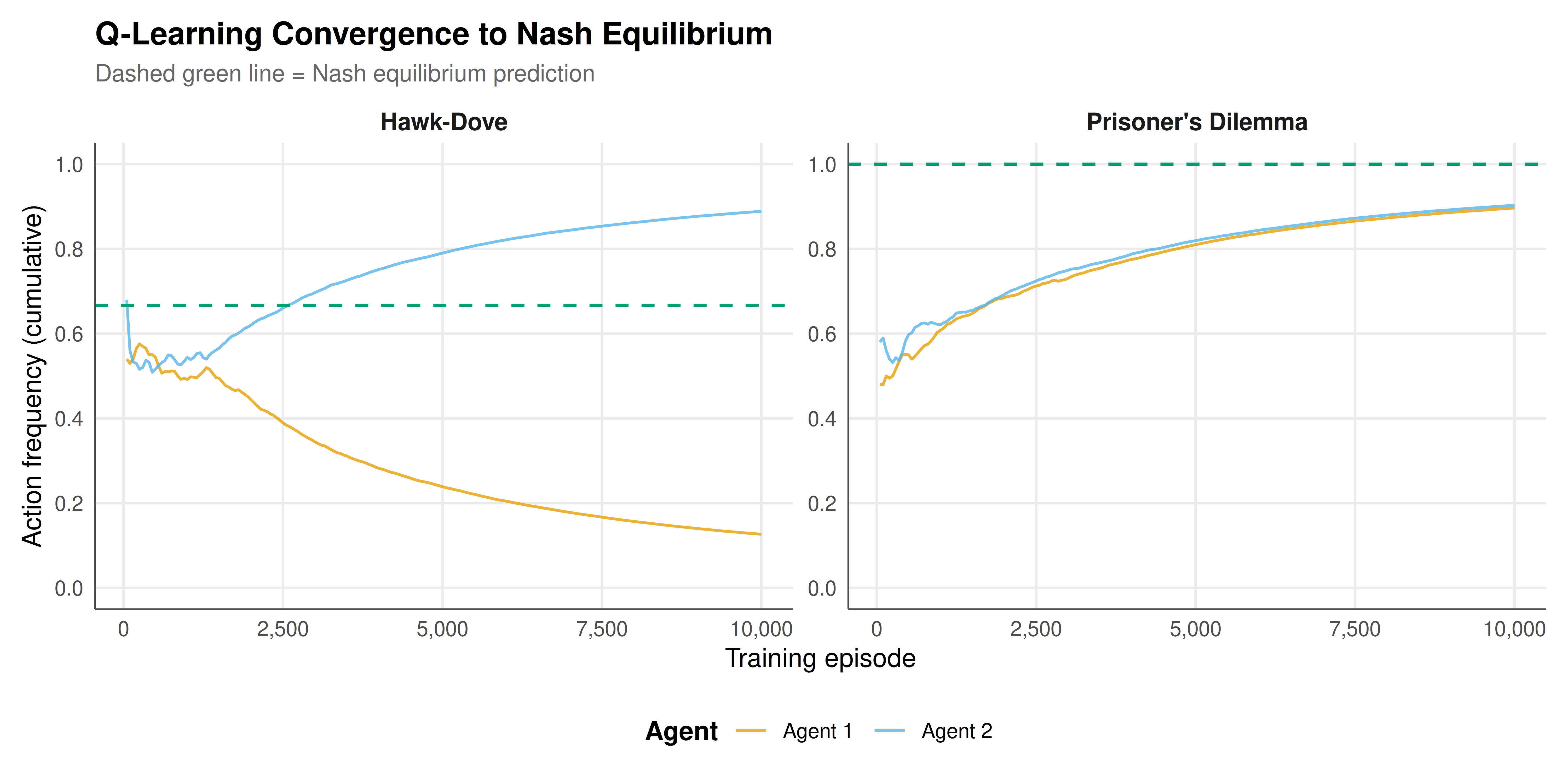
#| fig-cap: "Q-learning convergence in two game environments. Left: In the Prisoner's Dilemma, both agents converge toward the dominant-strategy Nash equilibrium of Defect. Right: In Hawk-Dove, agents converge toward the mixed-strategy Nash equilibrium (Hawk with probability 2/3). Dashed horizontal lines indicate the Nash equilibrium prediction."
#| fig-width: 10
#| fig-height: 5
#| dev: [png, pdf]
#| dpi: 300
# Combine frequency data
pd_freq <- pd_result$freq_data |> mutate(game = "Prisoner's Dilemma")
hd_freq <- hd_result$freq_data |> mutate(game = "Hawk-Dove")

# Filter to the "aggressive" action for cleaner plot
pd_defect <- pd_freq |> filter(action == "Defect")
hd_hawk   <- hd_freq |> filter(action == "Hawk")

plot_data <- bind_rows(
  pd_defect |> mutate(action_label = "Pr(Defect)"),
  hd_hawk   |> mutate(action_label = "Pr(Hawk)")
)

# Nash equilibrium reference lines
nash_refs <- data.frame(
  game = c("Prisoner's Dilemma", "Hawk-Dove"),
  nash_prob = c(1.0, v_param / c_param),
  action_label = c("Pr(Defect)", "Pr(Hawk)")
)

p_static <- ggplot(plot_data,
                   aes(x = episode, y = frequency,
                       color = player, linetype = player)) +
  geom_line(linewidth = 0.6, alpha = 0.8) +
  geom_hline(data = nash_refs, aes(yintercept = nash_prob),
             linetype = "dashed", color = okabe_ito[3], linewidth = 0.7) +
  facet_wrap(~ game, scales = "free_y") +
  scale_color_manual(
    values = c("Agent 1" = okabe_ito[1], "Agent 2" = okabe_ito[2]),
    name = "Agent"
  ) +
  scale_linetype_manual(
    values = c("Agent 1" = "solid", "Agent 2" = "solid"),
    name = "Agent"
  ) +
  scale_x_continuous(
    name = "Training episode",
    labels = scales::comma_format()
  ) +
  scale_y_continuous(
    name = "Action frequency (cumulative)",
    limits = c(0, 1), breaks = seq(0, 1, 0.2)
  ) +
  labs(
    title = "Q-Learning Convergence to Nash Equilibrium",
    subtitle = "Dashed green line = Nash equilibrium prediction"
  ) +
  theme_publication() +
  theme(
    strip.text = element_text(face = "bold", size = 11),
    legend.title = element_text(face = "bold")
  )

p_static
```
## Interactive figure
```{r}
#| label: fig-convergence-interactive
#| fig-cap: "Interactive convergence plot. Hover to see action frequencies at each training checkpoint."
plot_data <- plot_data |>
  mutate(
    text = paste0(
      "Game: ", game,
      "\n", player,
      "\nEpisode: ", episode,
      "\n", action_label, " = ", round(frequency, 4)
    )
  )

p_int <- ggplot(plot_data,
                aes(x = episode, y = frequency, color = player,
                    text = text)) +
  geom_line(linewidth = 0.5, alpha = 0.8) +
  geom_hline(data = nash_refs, aes(yintercept = nash_prob),
             linetype = "dashed", color = okabe_ito[3], linewidth = 0.6) +
  facet_wrap(~ game, scales = "free_y") +
  scale_color_manual(
    values = c("Agent 1" = okabe_ito[1], "Agent 2" = okabe_ito[2]),
    name = "Agent"
  ) +
  scale_x_continuous(name = "Training episode") +
  scale_y_continuous(name = "Action frequency",
                     limits = c(0, 1)) +
  labs(title = "Q-Learning Convergence to Nash Equilibrium") +
  theme_publication() +
  theme(strip.text = element_text(face = "bold"))

ggplotly(p_int, tooltip = "text") |>
  config(displaylogo = FALSE,
         modeBarButtonsToRemove = c("select2d", "lasso2d"))
```
## Interpretation
The reinforcement learning experiments reveal how independent Q-learning agents discover equilibrium strategies through repeated interaction, providing computational evidence for the game-theoretic prediction that rational agents will converge to Nash equilibrium even when they start with no knowledge of the game's payoff structure or their opponent's strategy. The convergence patterns differ markedly between the two games, reflecting their fundamentally different strategic structures.
In the Prisoner's Dilemma, both agents converge rapidly and monotonically toward the dominant-strategy Nash equilibrium of mutual defection. The convergence trajectory shows a characteristic initial exploration phase (high epsilon) where both actions are played with roughly equal frequency, followed by a transition phase where the agents begin to favor Defect as their Q-values diverge, and finally a convergence phase where Defect is played almost exclusively. The speed of convergence reflects the strength of dominance: because Defect yields a higher payoff regardless of the opponent's action, the Q-value for Defect accumulates positive reward differentials from the very first episodes. By the time the exploration rate has decayed substantially, the Q-value advantage of Defect is large enough that the greedy policy selects it deterministically.
The Hawk-Dove game presents a qualitatively different convergence challenge. The Nash equilibrium is in mixed strategies, with each player choosing Hawk with probability $p^* = v/c = 2/3$. Q-learning agents, which maintain Q-values for each action and select according to an epsilon-greedy or softmax policy, must converge not to a deterministic action but to a specific mixing proportion. In practice, this convergence is noisier and slower than in the Prisoner's Dilemma, because the agents are not converging to a fixed action but rather to a statistical regularity in their action frequencies. The cumulative action frequencies (which average over the entire history) smooth out the episode-by-episode fluctuations and reveal the underlying trend toward the Nash equilibrium mixing probability.
The R6 class architecture provides several design advantages for this application. The `GameEnvironment` class maintains internal state (the history of actions and rewards) that persists across method calls, which is essential for tracking the evolution of play over time. The reference semantics of R6 mean that the `step()` method can modify the environment's history in place without the overhead of copying the entire object on each call, which is important for performance when running thousands of training episodes. The `render()` method provides a human-readable display of the most recent action and reward, facilitating debugging and interactive exploration.
The `QLearningAgent` class encapsulates the agent's learning state (Q-values, exploration rate, action counts) and learning algorithm (epsilon-greedy selection, Q-value update rule). By separating the agent from the environment, the architecture supports plug-and-play experimentation: different learning algorithms (e.g., policy gradient, fictitious play, experience-weighted attraction) can be implemented as alternative agent classes that conform to the same interface (select_action, update), and different games can be implemented as alternative environment classes that conform to the Gym interface (reset, step, render). This modularity is the key contribution of the OpenAI Gym design philosophy, and our R6 implementation preserves it fully.
Several important caveats apply to the interpretation of these results. First, the Q-learning agents in this tutorial are memoryless: they do not condition their actions on the history of play. In the iterated Prisoner's Dilemma, history-dependent strategies like Tit-for-Tat can sustain cooperation as a subgame perfect equilibrium when the discount factor is sufficiently high. Our memoryless agents cannot discover these cooperative equilibria, and their convergence to mutual defection reflects the structure of the stage game rather than the repeated game. Extending the framework to support history-dependent strategies would require expanding the state space to include past actions, increasing the dimensionality of the Q-table exponentially.
Second, the convergence to Nash equilibrium in our experiments is not guaranteed by theory. The convergence of independent Q-learners in general-sum games is an open research question, and counterexamples exist where Q-learning cycles rather than converges. The games we have chosen --- one with a dominant-strategy equilibrium and one with a unique symmetric mixed equilibrium --- are among the most favorable cases for convergence. In games with multiple equilibria, payoff-asymmetric games, or games with more than two actions, convergence behavior can be more complex and depend sensitively on the learning rate schedule, initial Q-values, and exploration strategy.
Third, the epsilon-greedy exploration strategy, while simple and effective, has limitations. The exploration rate decays deterministically over time, regardless of whether the agent has sufficiently explored all actions. More sophisticated exploration strategies (e.g., UCB-based exploration, Thompson sampling) can improve convergence speed and robustness. The framework's modular design makes it straightforward to implement and compare alternative exploration strategies.
The visualization of convergence trajectories as cumulative action frequencies is a standard approach in the multi-agent learning literature. The key diagnostic is whether the frequency curves flatten at values close to the Nash equilibrium prediction. Persistent oscillation or drift away from Nash would indicate failure to converge, while rapid flattening indicates efficient learning. The dashed reference line at the Nash prediction provides an immediate visual benchmark, and the interactive version allows precise inspection of the convergence trajectory at any training checkpoint.
## Extensions & related tutorials
- **Classical games**: For the game-theoretic foundations of Prisoner's Dilemma and Hawk-Dove, see the [Classical Games](../../classical-games/) section and @axelrod_1984.
- **Evolutionary game theory**: The replicator dynamics provide an alternative model of strategy adaptation; see the [Evolutionary Game Theory](../../evolutionary-gt/) tutorials.
- **S4 classes for game objects**: The [S4 Classes for Game Objects](../../r-package-development/s4-classes-game-objects/) tutorial provides a complementary object-oriented representation of games using S4 classes.
- **Simulation techniques**: For more advanced simulation frameworks, see the [Simulations](../../simulations/) section.
- **AI/ML foundations**: The [AI/ML Foundations](../../ai-ml-foundations-and-applications/) section covers neural network approaches to game theory that extend beyond tabular Q-learning.
## References
::: {#refs}
:::