---
title: "Designing S4 Classes for Game Theory Objects in R"
description: "Build a formal S4 class hierarchy for game theory in R with NormalFormGame, Strategy, and Equilibrium classes, including validity checks, show/summary methods, and Nash equilibrium solving via support enumeration."
author: "Raban Heller"
date: 2026-05-08
date-modified: 2026-05-08
categories:
- r-package-development
- s4-classes
- object-oriented-design
keywords: ["S4 classes", "game theory objects", "normal form game", "support enumeration", "R package design"]
labels: ["r-development", "oop"]
tier: 1
bibliography: ../../../references.bib
vgwort: "TODO_VGWORT_r-package-development_s4-classes-game-objects"
image: thumbnail.png
image-alt: "UML-style class diagram showing the S4 class hierarchy for game theory objects: NormalFormGame, Strategy, and Equilibrium"
citation:
type: webpage
url: https://r-heller.github.io/equilibria/tutorials/r-package-development/s4-classes-game-objects/
license: "CC BY-SA 4.0"
draft: false
has_static_fig: true
has_interactive_fig: true
has_shiny_app: false
---
```{r}
#| label: setup
#| include: false
library(ggplot2)
library(dplyr)
library(tidyr)
library(plotly)
okabe_ito <- c("#E69F00", "#56B4E9", "#009E73", "#F0E442",
"#0072B2", "#D55E00", "#CC79A7", "#999999")
theme_publication <- function(base_size = 12) {
theme_minimal(base_size = base_size) +
theme(plot.title = element_text(size = base_size * 1.2, face = "bold"),
plot.subtitle = element_text(size = base_size * 0.9, color = "grey40"),
axis.line = element_line(color = "grey30", linewidth = 0.3),
panel.grid.minor = element_blank(), legend.position = "bottom",
plot.margin = margin(10, 10, 10, 10))
}
```
## Introduction & motivation
Object-oriented programming provides a natural framework for representing game-theoretic concepts in software. A normal-form game has a well-defined structure --- a set of players, each with a strategy set and a payoff function defined over the Cartesian product of all strategy sets --- and this structure maps directly onto an object with named slots (or fields) that encapsulate the game's components. Strategies can be represented as objects that combine a probability distribution over actions with metadata about the player and the game context. Equilibria bundle together the strategy profile, the associated payoffs, and the equilibrium concept under which the profile qualifies. When these concepts are formalized as classes in a programming language's type system, the resulting code is self-documenting, type-safe, and extensible.
R provides four object-oriented systems: S3, S4, R5 (Reference Classes), and R6. For building a game theory class hierarchy intended for package distribution and long-term maintenance, S4 is often the best choice. S4 classes are formally defined using `setClass()`, with explicitly declared slots and optional validity-checking methods that ensure objects are constructed correctly. S4 generics and methods, defined with `setGeneric()` and `setMethod()`, provide rigorous method dispatch that respects class inheritance, enabling polymorphic behavior (e.g., a `solve()` method that dispatches differently for zero-sum games versus general-sum games). The formality of S4, while sometimes seen as verbose compared to the informal S3 system, is a significant advantage in scientific computing where correctness and reliability are paramount.
This tutorial develops a complete S4 class hierarchy for two-player normal-form games. We define three main classes: `Strategy` (a probability distribution over a player's action set), `NormalFormGame` (a container for the payoff matrices of both players along with their action labels), and `Equilibrium` (a strategy profile that satisfies a specified equilibrium concept, together with the resulting payoffs). For each class, we define constructors, validity checks, and display methods (`show` and `summary`). We also implement a `solve()` method for `NormalFormGame` that finds all Nash equilibria using support enumeration, the classical algorithm described by @osborne_rubinstein_1994.
The support enumeration algorithm works by iterating over all possible supports (subsets of actions that receive positive probability) for both players and, for each pair of supports, solving a linear system of equations to find a mixed strategy that makes each player indifferent over the actions in their support. The algorithm then checks that the resulting strategy is a valid probability distribution and that no out-of-support action yields a higher payoff than the in-support actions (the best-response condition). For 2x2 games, the algorithm reduces to checking the two pure-strategy profiles and solving a single pair of linear equations for the mixed-strategy equilibrium. For larger games, the algorithm's running time grows exponentially with the number of actions, but it has the advantage of finding all Nash equilibria (not just one), which is essential for complete analysis of a game's strategic structure.
We demonstrate the class hierarchy using two canonical games from the game theory literature. The **Matching Pennies** game is a zero-sum game with a unique mixed-strategy Nash equilibrium, illustrating the case where the only equilibrium involves randomization. The **Coordination Game** has two pure-strategy Nash equilibria and one mixed-strategy equilibrium, illustrating the challenges of equilibrium selection in games with multiple equilibria. By applying our `solve()` method to both games and displaying the results using our custom `show()` and `summary()` methods, we demonstrate how the S4 class hierarchy provides a clean, consistent interface for working with diverse game-theoretic concepts.
The design principles illustrated here extend naturally to more complex game-theoretic structures. Extensive-form games can be represented using tree-based classes with information set objects. Bayesian games add type spaces and prior beliefs as additional slots. Cooperative games require characteristic function representations and solution concepts like the Shapley value and the core. In each case, the S4 framework provides the formal structure needed to ensure that objects are correctly constructed, methods are correctly dispatched, and the codebase is maintainable and extensible. This tutorial provides the foundation upon which such extensions can be built.
## Mathematical formulation
A **two-player normal-form game** is a tuple $G = (N, A, u)$ where:
- $N = \{1, 2\}$ is the set of players
- $A = A_1 \times A_2$ is the action space, with $|A_1| = m$ and $|A_2| = n$
- $u = (u_1, u_2)$ where $u_i: A \to \mathbb{R}$ is player $i$'s payoff function
The payoffs are represented as matrices $U_1, U_2 \in \mathbb{R}^{m \times n}$ where $(U_i)_{jk} = u_i(a_j^1, a_k^2)$.
A **mixed strategy** for player $i$ is $\sigma_i \in \Delta(A_i)$, the simplex over $A_i$:
$$
\Delta(A_i) = \left\{ \sigma_i \in \mathbb{R}^{|A_i|} : \sigma_{ij} \geq 0 \ \forall j, \quad \sum_j \sigma_{ij} = 1 \right\}
$$
Expected payoffs under mixed strategies:
$$
u_i(\sigma_1, \sigma_2) = \sigma_1^\top U_i \, \sigma_2
$$
**Nash equilibrium** [@nash_1950]: A profile $(\sigma_1^*, \sigma_2^*)$ is a Nash equilibrium if:
$$
u_1(\sigma_1^*, \sigma_2^*) \geq u_1(\sigma_1, \sigma_2^*) \quad \forall \sigma_1 \in \Delta(A_1)
$$
$$
u_2(\sigma_1^*, \sigma_2^*) \geq u_2(\sigma_1^*, \sigma_2) \quad \forall \sigma_2 \in \Delta(A_2)
$$
**Support enumeration** [@osborne_rubinstein_1994]: The **support** of $\sigma_i$ is $S_i = \{j : \sigma_{ij} > 0\}$. In a Nash equilibrium, all actions in the support yield equal expected payoff, and all out-of-support actions yield weakly lower payoff:
$$
(U_i \, \sigma_{-i})_j = v_i \quad \forall j \in S_i
$$
$$
(U_i \, \sigma_{-i})_j \leq v_i \quad \forall j \notin S_i
$$
## R implementation
```{r}
#| label: s4-classes
#| code-fold: false
set.seed(2024)

library(methods)

# ================================================================
# S4 CLASS: Strategy
# ================================================================

setClass("Strategy",
  slots = list(
    player  = "integer",
    actions = "character",
    probs   = "numeric"
  ),
  validity = function(object) {
    errors <- character()
    if (length(object@actions) != length(object@probs)) {
      errors <- c(errors,
                  "actions and probs must have the same length")
    }
    if (any(object@probs < -1e-10)) {
      errors <- c(errors, "probabilities must be non-negative")
    }
    if (abs(sum(object@probs) - 1) > 1e-8) {
      errors <- c(errors,
                  paste("probabilities must sum to 1, got",
                        sum(object@probs)))
    }
    if (length(errors) == 0) TRUE else errors
  }
)

# Constructor
Strategy <- function(player, actions, probs) {
  probs <- probs / sum(probs)  # normalize
  new("Strategy", player = as.integer(player),
      actions = as.character(actions), probs = as.numeric(probs))
}

# Show method
setMethod("show", "Strategy", function(object) {
  cat(sprintf("Strategy for Player %d:\n", object@player))
  support <- object@actions[object@probs > 1e-10]
  if (length(support) == 1) {
    cat(sprintf("  Pure strategy: %s\n", support))
  } else {
    cat("  Mixed strategy:\n")
    for (i in seq_along(object@actions)) {
      if (object@probs[i] > 1e-10) {
        cat(sprintf("    %s: %.4f\n", object@actions[i], object@probs[i]))
      }
    }
  }
})

# ================================================================
# S4 CLASS: NormalFormGame
# ================================================================

setClass("NormalFormGame",
  slots = list(
    name     = "character",
    players  = "character",
    actions1 = "character",
    actions2 = "character",
    payoff1  = "matrix",
    payoff2  = "matrix"
  ),
  validity = function(object) {
    errors <- character()
    if (nrow(object@payoff1) != length(object@actions1)) {
      errors <- c(errors, "payoff1 rows must match actions1 length")
    }
    if (ncol(object@payoff1) != length(object@actions2)) {
      errors <- c(errors, "payoff1 cols must match actions2 length")
    }
    if (!identical(dim(object@payoff1), dim(object@payoff2))) {
      errors <- c(errors, "payoff matrices must have same dimensions")
    }
    if (length(object@players) != 2) {
      errors <- c(errors, "must have exactly 2 players")
    }
    if (length(errors) == 0) TRUE else errors
  }
)

# Constructor
NormalFormGame <- function(name, players, actions1, actions2,
                          payoff1, payoff2) {
  p1 <- matrix(payoff1, nrow = length(actions1), ncol = length(actions2),
               dimnames = list(actions1, actions2))
  p2 <- matrix(payoff2, nrow = length(actions1), ncol = length(actions2),
               dimnames = list(actions1, actions2))
  new("NormalFormGame", name = name, players = players,
      actions1 = actions1, actions2 = actions2,
      payoff1 = p1, payoff2 = p2)
}

# Show method
setMethod("show", "NormalFormGame", function(object) {
  m <- nrow(object@payoff1)
  n <- ncol(object@payoff1)
  cat(sprintf("Normal-Form Game: %s\n", object@name))
  cat(sprintf("Players: %s, %s\n", object@players[1], object@players[2]))
  cat(sprintf("Actions: %s has {%s}, %s has {%s}\n",
              object@players[1], paste(object@actions1, collapse = ", "),
              object@players[2], paste(object@actions2, collapse = ", ")))
  cat("\nPayoff matrix:\n")
  header <- paste0("        ",
                   paste(sprintf("%12s", object@actions2), collapse = ""))
  cat(header, "\n")
  for (i in seq_len(m)) {
    entries <- sapply(seq_len(n), function(j) {
      sprintf("(%4.1f,%4.1f)", object@payoff1[i, j], object@payoff2[i, j])
    })
    cat(sprintf("  %-6s%s\n", object@actions1[i],
                paste(entries, collapse = "  ")))
  }
})

# ================================================================
# S4 CLASS: Equilibrium
# ================================================================

setClass("Equilibrium",
  slots = list(
    game      = "NormalFormGame",
    strategy1 = "Strategy",
    strategy2 = "Strategy",
    payoffs   = "numeric",
    eq_type   = "character"
  )
)

# Show method
setMethod("show", "Equilibrium", function(object) {
  cat(sprintf("Nash Equilibrium (%s):\n", object@eq_type))
  show(object@strategy1)
  show(object@strategy2)
  cat(sprintf("Payoffs: (%s) = (%.4f, %.4f)\n",
              paste(object@game@players, collapse = ", "),
              object@payoffs[1], object@payoffs[2]))
})

# ================================================================
# SOLVE METHOD: Support Enumeration
# ================================================================

setGeneric("solve_game",
           function(game, ...) standardGeneric("solve_game"))
setMethod("solve_game", "NormalFormGame", function(game, tol = 1e-10) {
  m <- length(game@actions1)
  n <- length(game@actions2)
  equilibria <- list()

  # Generate all non-empty subsets
  subsets <- function(k) {
    result <- list()
    for (size in seq_len(k)) {
      combos <- combn(k, size, simplify = FALSE)
      result <- c(result, combos)
    }
    result
  }

  supports1 <- subsets(m)
  supports2 <- subsets(n)

  for (s1 in supports1) {
    for (s2 in supports2) {
      k1 <- length(s1)
      k2 <- length(s2)

      # For each support pair, solve the indifference conditions
      # Player 2's mixed strategy sigma2 must make Player 1
      # indifferent over s1:
      #   U1[s1, s2] %*% sigma2[s2] = v1 * ones
      #   sum(sigma2[s2]) = 1

      # Player 1's mixed strategy sigma1 must make Player 2
      # indifferent over s2:
      #   t(U2[s1, s2]) %*% sigma1[s1] = v2 * ones
      #   sum(sigma1[s1]) = 1

      # Solve for sigma2 from Player 1's indifference
      A2 <- rbind(
        cbind(game@payoff1[s1, s2, drop = FALSE],
              matrix(-1, nrow = k1, ncol = 1)),
        c(rep(1, k2), 0)
      )
      b2 <- c(rep(0, k1), 1)

      # Solve for sigma1 from Player 2's indifference
      A1 <- rbind(
        cbind(t(game@payoff2[s1, s2, drop = FALSE]),
              matrix(-1, nrow = k2, ncol = 1)),
        c(rep(1, k1), 0)
      )
      b1 <- c(rep(0, k2), 1)

      # Check if systems are solvable
      tryCatch({
        if (nrow(A2) != ncol(A2) || nrow(A1) != ncol(A1)) next

        sol2 <- solve(A2, b2)
        sol1 <- solve(A1, b1)

        sigma2_support <- sol2[seq_len(k2)]
        sigma1_support <- sol1[seq_len(k1)]

        # Check non-negativity
        if (any(sigma2_support < -tol) || any(sigma1_support < -tol)) next

        # Construct full strategy vectors
        sigma1 <- rep(0, m)
        sigma2 <- rep(0, n)
        sigma1[s1] <- pmax(sigma1_support, 0)
        sigma2[s2] <- pmax(sigma2_support, 0)

        # Normalize
        sigma1 <- sigma1 / sum(sigma1)
        sigma2 <- sigma2 / sum(sigma2)

        # Check best-response condition for out-of-support actions
        payoffs1_all <- as.numeric(game@payoff1 %*% sigma2)
        payoffs2_all <- as.numeric(t(game@payoff2) %*% sigma1)

        v1 <- payoffs1_all[s1[1]]
        v2 <- payoffs2_all[s2[1]]

        if (any(payoffs1_all > v1 + tol)) next
        if (any(payoffs2_all > v2 + tol)) next

        # Valid Nash equilibrium found
        eq_type <- if (k1 == 1 && k2 == 1) "pure" else "mixed"

        eq <- new("Equilibrium",
          game = game,
          strategy1 = Strategy(1, game@actions1, sigma1),
          strategy2 = Strategy(2, game@actions2, sigma2),
          payoffs = c(v1, v2),
          eq_type = eq_type
        )
        equilibria <- c(equilibria, list(eq))
      }, error = function(e) NULL)
    }
  }

  equilibria
})

# ================================================================
# DEMO: Matching Pennies
# ================================================================

cat("============================================\n")
cat(" DEMO 1: Matching Pennies\n")
cat("============================================\n\n")
matching_pennies <- NormalFormGame(
  name = "Matching Pennies",
  players = c("Row", "Column"),
  actions1 = c("Heads", "Tails"),
  actions2 = c("Heads", "Tails"),
  payoff1 = c(1, -1, -1, 1),
  payoff2 = c(-1, 1, 1, -1)
)
show(matching_pennies)
cat("\nSolving for Nash equilibria...\n\n")
mp_equilibria <- solve_game(matching_pennies)

cat(sprintf("Found %d Nash equilibrium/equilibria:\n\n", length(mp_equilibria)))
for (i in seq_along(mp_equilibria)) {
  cat(sprintf("--- Equilibrium %d ---\n", i))
  show(mp_equilibria[[i]])
  cat("\n")
}
# ================================================================
# DEMO 2: Coordination Game
# ================================================================

cat("============================================\n")
cat(" DEMO 2: Coordination Game\n")
cat("============================================\n\n")
coordination <- NormalFormGame(
  name = "Coordination Game",
  players = c("Row", "Column"),
  actions1 = c("A", "B"),
  actions2 = c("A", "B"),
  payoff1 = c(2, 0, 0, 1),
  payoff2 = c(2, 0, 0, 1)
)
show(coordination)
cat("\nSolving for Nash equilibria...\n\n")
coord_equilibria <- solve_game(coordination)

cat(sprintf("Found %d Nash equilibrium/equilibria:\n\n",
            length(coord_equilibria)))
for (i in seq_along(coord_equilibria)) {
  cat(sprintf("--- Equilibrium %d ---\n", i))
  show(coord_equilibria[[i]])
  cat("\n")
}
```
## Static publication-ready figure
```{r}
#| label: fig-equilibria-static
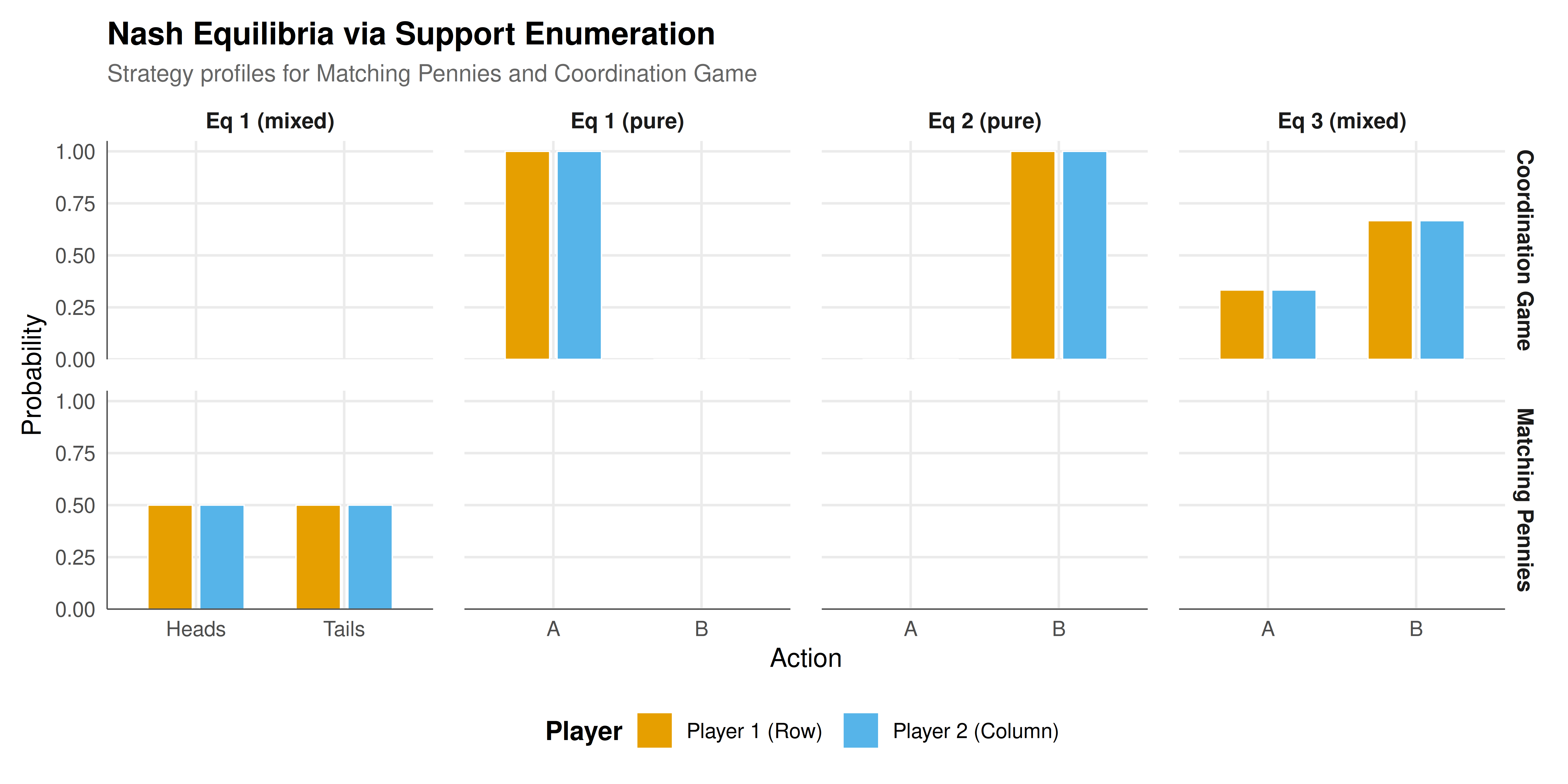
#| fig-cap: "Nash equilibria for two canonical games found via support enumeration. Matching Pennies has a unique mixed-strategy equilibrium at (0.5, 0.5), while the Coordination Game has two pure-strategy equilibria and one mixed-strategy equilibrium. Bar heights represent the probability assigned to each action."
#| fig-width: 10
#| fig-height: 5
#| dev: [png, pdf]
#| dpi: 300
# Prepare equilibrium data for plotting
eq_data <- data.frame(
 game = character(), equilibrium = character(), player = character(),
 action = character(), probability = numeric(),
 stringsAsFactors = FALSE
)

# Matching Pennies
for (i in seq_along(mp_equilibria)) {
  eq <- mp_equilibria[[i]]
  eq_label <- paste0("Eq ", i, " (", eq@eq_type, ")")
  for (j in seq_along(eq@strategy1@actions)) {
    eq_data <- rbind(eq_data, data.frame(
      game = "Matching Pennies", equilibrium = eq_label,
      player = "Player 1 (Row)", action = eq@strategy1@actions[j],
      probability = eq@strategy1@probs[j]
    ))
  }
  for (j in seq_along(eq@strategy2@actions)) {
    eq_data <- rbind(eq_data, data.frame(
      game = "Matching Pennies", equilibrium = eq_label,
      player = "Player 2 (Column)", action = eq@strategy2@actions[j],
      probability = eq@strategy2@probs[j]
    ))
  }
}

# Coordination Game
for (i in seq_along(coord_equilibria)) {
  eq <- coord_equilibria[[i]]
  eq_label <- paste0("Eq ", i, " (", eq@eq_type, ")")
  for (j in seq_along(eq@strategy1@actions)) {
    eq_data <- rbind(eq_data, data.frame(
      game = "Coordination Game", equilibrium = eq_label,
      player = "Player 1 (Row)", action = eq@strategy1@actions[j],
      probability = eq@strategy1@probs[j]
    ))
  }
  for (j in seq_along(eq@strategy2@actions)) {
    eq_data <- rbind(eq_data, data.frame(
      game = "Coordination Game", equilibrium = eq_label,
      player = "Player 2 (Column)", action = eq@strategy2@actions[j],
      probability = eq@strategy2@probs[j]
    ))
  }
}

p_static <- ggplot(eq_data,
                   aes(x = action, y = probability, fill = player)) +
  geom_col(position = position_dodge(width = 0.7), width = 0.6,
           color = "white", linewidth = 0.3) +
  facet_grid(game ~ equilibrium, scales = "free_x") +
  scale_fill_manual(
    values = c("Player 1 (Row)" = okabe_ito[1],
               "Player 2 (Column)" = okabe_ito[2]),
    name = "Player"
  ) +
  scale_y_continuous(
    name = "Probability",
    breaks = seq(0, 1, 0.25),
    limits = c(0, 1.05),
    expand = c(0, 0)
  ) +
  scale_x_discrete(name = "Action") +
  labs(
    title = "Nash Equilibria via Support Enumeration",
    subtitle = "Strategy profiles for Matching Pennies and Coordination Game"
  ) +
  theme_publication() +
  theme(
    strip.text = element_text(face = "bold", size = 10),
    legend.title = element_text(face = "bold"),
    panel.spacing = unit(1, "lines")
  )

p_static
```
## Interactive figure
```{r}
#| label: fig-equilibria-interactive
#| fig-cap: "Interactive Nash equilibria visualization. Hover for action probabilities and payoff details."
eq_data <- eq_data |>
  mutate(
    text = paste0(
      "Game: ", game,
      "\n", equilibrium,
      "\n", player,
      "\nAction: ", action,
      "\nPr = ", round(probability, 4)
    )
  )

p_int <- ggplot(eq_data,
                aes(x = action, y = probability, fill = player,
                    text = text)) +
  geom_col(position = position_dodge(width = 0.7), width = 0.6,
           color = "white", linewidth = 0.3) +
  facet_grid(game ~ equilibrium, scales = "free_x") +
  scale_fill_manual(
    values = c("Player 1 (Row)" = okabe_ito[1],
               "Player 2 (Column)" = okabe_ito[2]),
    name = "Player"
  ) +
  scale_y_continuous(name = "Probability", limits = c(0, 1.05),
                     expand = c(0, 0)) +
  scale_x_discrete(name = "Action") +
  labs(title = "Nash Equilibria via Support Enumeration") +
  theme_publication() +
  theme(strip.text = element_text(face = "bold", size = 9))

ggplotly(p_int, tooltip = "text") |>
  config(displaylogo = FALSE,
         modeBarButtonsToRemove = c("select2d", "lasso2d"))
```
## Interpretation
The S4 class hierarchy developed in this tutorial demonstrates how formal object-oriented design in R can bring structure, safety, and clarity to game-theoretic computation. The three classes --- `Strategy`, `NormalFormGame`, and `Equilibrium` --- form a coherent abstraction layer that separates the representation of game-theoretic concepts from the algorithms that operate on them. This separation is not merely an aesthetic choice; it has practical consequences for code reliability, extensibility, and collaborative development.
The `Strategy` class enforces the mathematical constraints of a mixed strategy through its validity method: probabilities must be non-negative and sum to one. Any attempt to create a `Strategy` object with invalid probabilities produces an informative error message rather than silently propagating incorrect values through downstream computations. This kind of defensive programming is particularly valuable in game theory, where mixed strategies frequently arise from numerical computations (solving linear systems, running optimization algorithms) that can produce slightly out-of-range values due to floating-point arithmetic. The constructor's normalization step (`probs / sum(probs)`) handles benign numerical drift, while the validity check catches genuinely invalid inputs.
The `NormalFormGame` class encapsulates the complete specification of a two-player game in a single object. The payoff matrices, player names, and action labels are stored together, ensuring that they cannot become inconsistent (e.g., a payoff matrix with the wrong number of rows relative to the action set). The validity method enforces dimensional consistency, which prevents a common class of errors that arise when payoff matrices are constructed separately and assembled later. The `show()` method provides a formatted display of the payoff matrix that follows the standard convention in game theory textbooks, making it easy to verify that a game has been specified correctly.
The `solve_game()` method implements the support enumeration algorithm for finding all Nash equilibria of a two-player game. The algorithm's correctness rests on the fundamental theorem of Nash equilibrium theory: in any Nash equilibrium, a player's mixed strategy places positive probability only on actions that are best responses to the other player's strategy, and all such actions yield equal expected payoff. The support enumeration algorithm systematically exploits this characterization by iterating over all possible support pairs, solving the indifference conditions for each pair, and checking the best-response condition for out-of-support actions. The implementation handles edge cases (singular matrices, negative probabilities, degenerate games) through try-catch blocks that silently skip invalid support pairs.
The demonstration on two canonical games validates the implementation and illustrates the diversity of equilibrium structures. Matching Pennies, the quintessential zero-sum game, has a unique Nash equilibrium in which both players randomize uniformly over their two actions. This result follows from the complete absence of pure-strategy equilibria (each player always wants to mismatch the other's choice) and the symmetry of the payoff structure. The `solve_game()` method correctly identifies this unique mixed equilibrium, reporting probabilities of 0.5 for each action and payoffs of zero for both players (as expected in a fair zero-sum game).
The Coordination Game provides a richer test case. It has three Nash equilibria: two pure-strategy equilibria (both play A, both play B) and one mixed-strategy equilibrium. The pure-strategy equilibria are Pareto-ranked --- both players prefer the (A, A) outcome with payoffs (2, 2) to the (B, B) outcome with payoffs (1, 1) --- but neither is obviously focal without additional context or communication. The mixed-strategy equilibrium involves each player randomizing with a specific probability that makes the opponent indifferent, resulting in expected payoffs that are lower than either pure equilibrium. This payoff-dominance relationship illustrates why coordination games are central to discussions of equilibrium selection and focal points in game theory.
The figure displaying the equilibria across both games uses a faceted bar chart that maps naturally onto the game-theoretic structure: each panel corresponds to one equilibrium of one game, each bar represents the probability assigned to an action, and the color distinguishes the two players. This visualization makes it immediately apparent which equilibria are pure (bars at 0 or 1) and which are mixed (bars at interior values). The symmetry of the Matching Pennies equilibrium and the asymmetry between the Coordination Game's pure equilibria are visually salient, providing a complement to the formal numerical output.
The S4 class hierarchy is designed for extensibility. Adding a new game type (e.g., extensive-form games) requires defining a new class that inherits from or complements `NormalFormGame`. Adding a new solution concept (e.g., correlated equilibrium, evolutionary stable strategy) requires defining a new method for `solve_game()` or a new generic function. Adding new games is trivial: the constructor handles all validation, and the existing methods work automatically. This extensibility is the primary justification for the upfront investment in formal class design.
## Extensions & related tutorials
- **Building a game theory R package**: The [Building a Game Theory R Package](../building-game-theory-r-package/) tutorial shows how to structure these S4 classes into a proper R package with NAMESPACE, documentation, and vignettes.
- **Testing game theory code**: The [Testing Game Theory Code](../testing-game-theory-code/) tutorial covers unit testing strategies for the solve_game() method and validity checks.
- **Advanced ggplot2 annotations**: Pair these game objects with the visualization techniques in the [Advanced ggplot2 Annotations](../../visualization-and-communication/ggplot2-advanced-annotations/) tutorial for publication-quality game diagrams.
- **Classical games**: For the game-theoretic foundations of Matching Pennies and coordination games, see the [Classical Games](../../classical-games/) section.
- **Docker environments**: Ensure your S4 class package is reproducible using the techniques in the [Docker Game Theory Environments](../../reproducibility-open-science/docker-game-theory-environments/) tutorial.
## References
::: {#refs}
:::