---
title: "Accelerating Game Solvers with Rcpp and Optimised R"
description: "Profiling game-theoretic computations in R, implementing support enumeration and fictitious play, presenting Rcpp C++ code for acceleration, and benchmarking pure-R optimisation strategies for performance-critical solvers."
author: "Raban Heller"
date: 2026-05-08
date-modified: 2026-05-08
categories:
- r-package-development
- performance-optimisation
- rcpp
keywords: ["Rcpp", "performance", "support enumeration", "fictitious play", "benchmarking"]
labels: ["r-development", "performance"]
tier: 1
bibliography: ../../../references.bib
vgwort: "TODO_VGWORT_R_PKG_RCPP_SOLVERS"
image: thumbnail.png
image-alt: "Benchmark comparison of loop-based vs vectorised R for fictitious play convergence"
citation:
type: webpage
url: https://r-heller.github.io/equilibria/tutorials/r-package-development/rcpp-game-solvers/
license: "CC BY-SA 4.0"
draft: false
has_static_fig: true
has_interactive_fig: true
has_shiny_app: false
---
```{r}
#| label: setup
#| include: false
library(ggplot2)
library(dplyr)
library(tidyr)
library(plotly)
okabe_ito <- c("#E69F00", "#56B4E9", "#009E73", "#F0E442",
"#0072B2", "#D55E00", "#CC79A7", "#999999")
theme_publication <- function(base_size = 12) {
theme_minimal(base_size = base_size) +
theme(plot.title = element_text(size = base_size * 1.2, face = "bold"),
plot.subtitle = element_text(size = base_size * 0.9, color = "grey40"),
axis.line = element_line(color = "grey30", linewidth = 0.3),
panel.grid.minor = element_blank(), legend.position = "bottom",
plot.margin = margin(10, 10, 10, 10))
}
```
## Introduction & motivation
Game theory is computationally demanding. Finding Nash equilibria of even moderately sized games requires exploring exponentially many strategy combinations, solving systems of linear equations or inequalities, and iterating convergence procedures that may require thousands or millions of steps. While R excels at statistical modelling, data visualisation, and rapid prototyping, its performance characteristics — interpreted execution, copy-on-modify semantics, and limited native support for in-place mutation — can make it poorly suited for the tight loops and large-scale matrix operations that game-theoretic algorithms demand. Understanding where R is slow, why it is slow, and how to make it faster is essential for anyone building serious computational game theory tools in the R ecosystem.
This tutorial addresses three levels of performance optimisation for game-theoretic computations in R. The first level is **profiling and diagnosis**: identifying which parts of a computation are actually slow, as opposed to which parts we merely suspect are slow. Programmers' intuitions about performance bottlenecks are notoriously unreliable, and systematic measurement is the only way to guide optimisation efforts effectively. We use R's built-in timing tools to measure the performance of a support enumeration algorithm for finding Nash equilibria of bimatrix games, identifying the specific operations that dominate runtime.
The second level is **pure-R optimisation**: rewriting slow code to exploit R's vectorised operations, pre-allocating memory, and avoiding unnecessary copies. R's vectorisation is built on highly optimised C and Fortran routines for linear algebra (BLAS and LAPACK), so a well-vectorised R program can approach the performance of compiled code for many operations. We demonstrate this by implementing fictitious play — a classical algorithm for computing mixed-strategy Nash equilibria — in both a naive loop-based style and a vectorised style, and show the dramatic speedup that vectorisation provides.
The third level is **Rcpp integration**: writing critical inner loops in C++ and calling them from R. Rcpp, developed by Dirk Eddelbuettel and Romain Francois, provides seamless interoperability between R and C++, allowing developers to write performance-critical code in C++ while retaining R's expressive syntax for everything else. In this tutorial, we present the C++ code that would be used to accelerate our game solvers, explain its structure and logic, and show the expected speedup based on algorithmic analysis. However, because Rcpp compilation requires a C++ toolchain that may not be available in all rendering environments, we benchmark the pure-R equivalents and project the Rcpp speedup based on known performance ratios for similar operations.
The support enumeration algorithm, introduced by Mangasarian in 1964 and closely related to the Lemke-Howson method [@lemke_howson_1964], finds all Nash equilibria of a bimatrix game by systematically enumerating all possible support pairs (the sets of strategies that each player uses with positive probability). For each support pair, it solves a system of linear equations to find the mixing probabilities that make each player indifferent among the strategies in their opponent's support. This algorithm is complete (it finds all equilibria) but its runtime is exponential in the number of strategies, making it suitable only for small games. It is, however, an excellent test case for performance optimisation because the inner loop — solving a linear system for each support pair — is both well-defined and performance-critical.
Fictitious play, introduced by Brown in 1951 and proved to converge for certain game classes by Robinson in 1951, is an iterative algorithm where players repeatedly best-respond to the empirical frequency of their opponent's past actions. It converges to a Nash equilibrium for two-player zero-sum games and for games with special structure, and it provides a useful approximation in general. Its main computational cost is the best-response computation at each iteration, which involves a matrix-vector multiplication — an operation that benefits enormously from vectorisation and compiled code.
## Mathematical formulation
### Bimatrix game
A two-player normal-form game is defined by payoff matrices $A, B \in \mathbb{R}^{m \times n}$, where $A_{ij}$ is Player 1's payoff and $B_{ij}$ is Player 2's payoff when Player 1 plays row $i$ and Player 2 plays column $j$.
### Support enumeration
A **support** is a subset of strategies played with positive probability. For a Nash equilibrium $(p, q)$:
- $\text{supp}(p) = \{i : p_i > 0\}$, $\text{supp}(q) = \{j : q_j > 0\}$
- Player 2's mixture $q$ makes Player 1 indifferent over $\text{supp}(p)$:
$$
(Aq)_i = v_1 \quad \forall i \in \text{supp}(p)
$$
- Player 1's mixture $p$ makes Player 2 indifferent over $\text{supp}(q)$:
$$
(B^T p)_j = v_2 \quad \forall j \in \text{supp}(q)
$$
For each support pair $(S_1, S_2)$ with $|S_1| = |S_2| = k$, we solve:
$$
\begin{pmatrix} A_{S_1, S_2} \\ \mathbf{1}^T \end{pmatrix} q_{S_2} = \begin{pmatrix} v_1 \cdot \mathbf{1} \\ 1 \end{pmatrix}
$$
### Fictitious play
At iteration $t$, each player best-responds to the opponent's empirical strategy:
$$
\bar{q}^{(t)} = \frac{1}{t} \sum_{\tau=1}^{t} e_{j_\tau}, \quad i_{t+1} = \arg\max_i (A \bar{q}^{(t)})_i
$$
The **exploitability** measures convergence:
$$
\epsilon(t) = \max_i (A \bar{q}^{(t)})_i + \max_j (B^T \bar{p}^{(t)})_j - \bar{p}^{(t)T} A \bar{q}^{(t)} - \bar{p}^{(t)T} B \bar{q}^{(t)}
$$
### Complexity
- **Support enumeration**: $O\left(\sum_{k=1}^{\min(m,n)} \binom{m}{k}\binom{n}{k} \cdot k^3\right)$ — exponential in game size.
- **Fictitious play per iteration**: $O(mn)$ for the matrix-vector product.
- **Rcpp speedup factor**: typically $10\text{-}100\times$ for loop-heavy code, $2\text{-}5\times$ for already-vectorised code.
## R implementation
```{r}
#| label: implementation
set.seed(2026)

# ============================================================
# PART 1: Support Enumeration in Pure R
# ============================================================

# --- Generate subsets of size k from 1:n ---
combn_list <- function(n, k) {
  if (k > n || k < 1) return(list())
  as.list(as.data.frame(combn(n, k)))
}

# --- Support enumeration solver ---
support_enumeration <- function(A, B, tol = 1e-10) {
  m <- nrow(A)
  n <- ncol(A)
  equilibria <- list()

  for (k in 1:min(m, n)) {
    supports_1 <- combn_list(m, k)
    supports_2 <- combn_list(n, k)

    for (s1 in supports_1) {
      for (s2 in supports_2) {
        # Solve for q: A[s1, s2] %*% q = v1 * 1, sum(q) = 1
        A_sub <- A[s1, s2, drop = FALSE]
        B_sub <- B[s1, s2, drop = FALSE]

        # Augmented system for q
        M_q <- rbind(A_sub, rep(1, k))
        # We need to find q and v1 such that A_sub %*% q = v1 * 1, sum(q) = 1
        # Rewrite: [A_sub, -1] [q; v1] = [0; ...], [1,...,1, 0] [q; v1] = 1
        if (k == 1) {
          q <- 1
          v1 <- A_sub[1, 1]
        } else {
          M <- rbind(
            cbind(A_sub, -rep(1, k)),
            c(rep(1, k), 0)
          )
          rhs <- c(rep(0, k), 1)
          sol_q <- tryCatch(solve(M, rhs), error = function(e) NULL)
          if (is.null(sol_q)) next
          q <- sol_q[1:k]
          v1 <- sol_q[k + 1]
        }

        # Solve for p: B[s1, s2]^T %*% p = v2 * 1, sum(p) = 1
        if (k == 1) {
          p <- 1
          v2 <- B_sub[1, 1]
        } else {
          M2 <- rbind(
            cbind(t(B_sub), -rep(1, k)),
            c(rep(1, k), 0)
          )
          rhs2 <- c(rep(0, k), 1)
          sol_p <- tryCatch(solve(M2, rhs2), error = function(e) NULL)
          if (is.null(sol_p)) next
          p <- sol_p[1:k]
          v2 <- sol_p[k + 1]
        }

        # Check: all probabilities non-negative
        if (any(p < -tol) || any(q < -tol)) next

        # Check: strategies outside support give lower payoff
        p_full <- rep(0, m); p_full[s1] <- pmax(p, 0)
        q_full <- rep(0, n); q_full[s2] <- pmax(q, 0)

        payoffs_1 <- A %*% q_full
        payoffs_2 <- t(B) %*% p_full

        if (any(payoffs_1[-s1] > v1 + tol)) next
        if (any(payoffs_2[-s2] > v2 + tol)) next

        equilibria[[length(equilibria) + 1]] <- list(
          p = p_full, q = q_full,
          v1 = v1, v2 = v2,
          support_1 = s1, support_2 = s2
        )
      }
    }
  }
  equilibria
}

# --- Test on a 3x3 game ---
A <- matrix(c(3, 0, 5, 4, 5, 1, 0, 3, 2), nrow = 3, byrow = TRUE)
B <- matrix(c(3, 5, 0, 1, 5, 4, 2, 3, 0), nrow = 3, byrow = TRUE)

cat("Payoff matrix A (Player 1):\n")
print(A)
cat("\nPayoff matrix B (Player 2):\n")
print(B)
ne <- support_enumeration(A, B)
cat("\nNash equilibria found:", length(ne), "\n")
for (i in seq_along(ne)) {
  cat("\nEquilibrium", i, ":\n")
  cat("  p =", round(ne[[i]]$p, 4), "\n")
  cat("  q =", round(ne[[i]]$q, 4), "\n")
  cat("  Payoffs: (", round(ne[[i]]$v1, 4), ",", round(ne[[i]]$v2, 4), ")\n")
}
# ============================================================
# PART 2: Benchmarking support enumeration across game sizes
# ============================================================

benchmark_se <- function(sizes, n_reps = 3) {
  results <- data.frame(
    size = integer(), time_ms = numeric(), n_equilibria = integer()
  )

  for (sz in sizes) {
    times <- numeric(n_reps)
    n_eq <- 0
    for (rep in 1:n_reps) {
      A_rand <- matrix(runif(sz^2, 0, 10), nrow = sz)
      B_rand <- matrix(runif(sz^2, 0, 10), nrow = sz)
      t0 <- proc.time()
      eq <- support_enumeration(A_rand, B_rand)
      times[rep] <- (proc.time() - t0)[3] * 1000  # milliseconds
      n_eq <- length(eq)
    }
    results <- rbind(results, data.frame(
      size = sz, time_ms = mean(times), n_equilibria = n_eq
    ))
  }
  results
}

sizes <- 2:6
cat("\n=== Benchmarking Support Enumeration ===\n")
se_bench <- benchmark_se(sizes)
print(se_bench)
# ============================================================
# PART 3: Fictitious Play — Naive vs Vectorised
# ============================================================

# --- Naive (loop-based) fictitious play ---
fictitious_play_naive <- function(A, B, n_iter = 2000) {
  m <- nrow(A); n <- ncol(A)
  counts_1 <- rep(0, m)  # action counts for player 1
  counts_2 <- rep(0, n)  # action counts for player 2

  exploitability <- numeric(n_iter)

  for (t in 1:n_iter) {
    # Empirical strategies
    p_bar <- if (sum(counts_1) > 0) counts_1 / sum(counts_1) else rep(1/m, m)
    q_bar <- if (sum(counts_2) > 0) counts_2 / sum(counts_2) else rep(1/n, n)

    # Best responses (computed element-by-element)
    payoffs_1 <- numeric(m)
    for (i in 1:m) {
      for (j in 1:n) {
        payoffs_1[i] <- payoffs_1[i] + A[i, j] * q_bar[j]
      }
    }
    br_1 <- which.max(payoffs_1)

    payoffs_2 <- numeric(n)
    for (j in 1:n) {
      for (i in 1:m) {
        payoffs_2[j] <- payoffs_2[j] + B[i, j] * p_bar[i]
      }
    }
    br_2 <- which.max(payoffs_2)

    counts_1[br_1] <- counts_1[br_1] + 1
    counts_2[br_2] <- counts_2[br_2] + 1

    # Exploitability
    exploitability[t] <- max(payoffs_1) + max(payoffs_2) -
      sum(p_bar * (A %*% q_bar)) - sum(q_bar * (t(B) %*% p_bar))
  }

  list(p = counts_1 / sum(counts_1),
       q = counts_2 / sum(counts_2),
       exploitability = exploitability)
}

# --- Vectorised fictitious play ---
fictitious_play_vec <- function(A, B, n_iter = 2000) {
  m <- nrow(A); n <- ncol(A)
  counts_1 <- rep(0, m)
  counts_2 <- rep(0, n)

  exploitability <- numeric(n_iter)

  for (t in 1:n_iter) {
    p_bar <- if (sum(counts_1) > 0) counts_1 / sum(counts_1) else rep(1/m, m)
    q_bar <- if (sum(counts_2) > 0) counts_2 / sum(counts_2) else rep(1/n, n)

    # Vectorised best responses
    payoffs_1 <- as.vector(A %*% q_bar)
    br_1 <- which.max(payoffs_1)

    payoffs_2 <- as.vector(t(B) %*% p_bar)
    br_2 <- which.max(payoffs_2)

    counts_1[br_1] <- counts_1[br_1] + 1
    counts_2[br_2] <- counts_2[br_2] + 1

    exploitability[t] <- max(payoffs_1) + max(payoffs_2) -
      sum(p_bar * (A %*% q_bar)) - sum(q_bar * (t(B) %*% p_bar))
  }

  list(p = counts_1 / sum(counts_1),
       q = counts_2 / sum(counts_2),
       exploitability = exploitability)
}

# --- Benchmark comparison ---
cat("\n=== Fictitious Play Benchmark ===\n")
game_sizes <- c(5, 10, 20, 50)
fp_bench <- data.frame(
  size = integer(), method = character(), time_ms = numeric()
)

for (sz in game_sizes) {
  A_test <- matrix(runif(sz^2, 0, 10), nrow = sz)
  B_test <- matrix(runif(sz^2, 0, 10), nrow = sz)
  n_it <- 1000

  t_naive <- system.time(fictitious_play_naive(A_test, B_test, n_it))[3] * 1000
  t_vec <- system.time(fictitious_play_vec(A_test, B_test, n_it))[3] * 1000

  fp_bench <- rbind(fp_bench,
    data.frame(size = sz, method = "Naive (loops)", time_ms = t_naive),
    data.frame(size = sz, method = "Vectorised", time_ms = t_vec)
  )
}

fp_bench$speedup <- NA
for (sz in game_sizes) {
  t_naive <- fp_bench$time_ms[fp_bench$size == sz & fp_bench$method == "Naive (loops)"]
  t_vec <- fp_bench$time_ms[fp_bench$size == sz & fp_bench$method == "Vectorised"]
  fp_bench$speedup[fp_bench$size == sz & fp_bench$method == "Vectorised"] <-
    round(t_naive / t_vec, 1)
}

cat("\nFictitious play timing (1000 iterations):\n")
print(fp_bench)
# --- Convergence analysis ---
A_conv <- matrix(c(0, -1, 1, 1, 0, -1, -1, 1, 0), nrow = 3, byrow = TRUE)
B_conv <- -A_conv  # zero-sum: Rock-Paper-Scissors

fp_result <- fictitious_play_vec(A_conv, B_conv, n_iter = 5000)
cat("\n=== Rock-Paper-Scissors Convergence ===\n")
cat("Final strategy p:", round(fp_result$p, 4), "\n")
cat("Final strategy q:", round(fp_result$q, 4), "\n")
cat("Final exploitability:", round(tail(fp_result$exploitability, 1), 6), "\n")
cat("Theoretical NE: (1/3, 1/3, 1/3)\n")
# ============================================================
# PART 4: Rcpp C++ Code (shown but not compiled)
# ============================================================

cat("\n=== Rcpp C++ Code for Fictitious Play ===\n")
cat("The following C++ code can be compiled with Rcpp::sourceCpp()\n")
cat("for approximately 10-50x speedup over the naive R version:\n\n")
rcpp_code <- '
#include <Rcpp.h>
using namespace Rcpp;

// [[Rcpp::export]]
List fictitious_play_cpp(NumericMatrix A, NumericMatrix B, int n_iter) {
  int m = A.nrow(), n = A.ncol();
  NumericVector counts_1(m, 0.0), counts_2(n, 0.0);
  NumericVector exploitability(n_iter);

  for (int t = 0; t < n_iter; t++) {
    double sum1 = 0, sum2 = 0;
    for (int i = 0; i < m; i++) sum1 += counts_1[i];
    for (int j = 0; j < n; j++) sum2 += counts_2[j];

    NumericVector p_bar(m), q_bar(n);
    for (int i = 0; i < m; i++)
      p_bar[i] = (sum1 > 0) ? counts_1[i] / sum1 : 1.0 / m;
    for (int j = 0; j < n; j++)
      q_bar[j] = (sum2 > 0) ? counts_2[j] / sum2 : 1.0 / n;

    // Best response for player 1: argmax_i sum_j A[i,j] * q_bar[j]
    int br_1 = 0;
    double max_pay_1 = -1e30;
    for (int i = 0; i < m; i++) {
      double pay = 0;
      for (int j = 0; j < n; j++) pay += A(i, j) * q_bar[j];
      if (pay > max_pay_1) { max_pay_1 = pay; br_1 = i; }
    }

    // Best response for player 2: argmax_j sum_i B[i,j] * p_bar[i]
    int br_2 = 0;
    double max_pay_2 = -1e30;
    for (int j = 0; j < n; j++) {
      double pay = 0;
      for (int i = 0; i < m; i++) pay += B(i, j) * p_bar[i];
      if (pay > max_pay_2) { max_pay_2 = pay; br_2 = j; }
    }

    counts_1[br_1] += 1;
    counts_2[br_2] += 1;

    // Compute exploitability
    double val_1 = 0, val_2 = 0;
    for (int i = 0; i < m; i++)
      for (int j = 0; j < n; j++) {
        val_1 += p_bar[i] * A(i, j) * q_bar[j];
        val_2 += p_bar[i] * B(i, j) * q_bar[j];
      }
    exploitability[t] = max_pay_1 + max_pay_2 - val_1 - val_2;
  }

  // Normalise
  double total_1 = 0, total_2 = 0;
  for (int i = 0; i < m; i++) total_1 += counts_1[i];
  for (int j = 0; j < n; j++) total_2 += counts_2[j];
  for (int i = 0; i < m; i++) counts_1[i] /= total_1;
  for (int j = 0; j < n; j++) counts_2[j] /= total_2;

  return List::create(
    Named("p") = counts_1,
    Named("q") = counts_2,
    Named("exploitability") = exploitability
  );
}
'
cat(rcpp_code)
# Projected Rcpp speedup
cat("\n=== Projected Rcpp Speedups ===\n")
projected <- fp_bench |>
  filter(method == "Naive (loops)") |>
  mutate(
    projected_rcpp_ms = time_ms / 30,  # conservative 30x speedup
    method = "Projected Rcpp"
  )
cat("Based on typical Rcpp speedup factors (10-50x over loop-based R):\n")
for (i in seq_len(nrow(projected))) {
  cat(sprintf("  %dx%d game: %.1f ms (R naive) -> %.1f ms (Rcpp projected)\n",
              projected$size[i], projected$size[i],
              fp_bench$time_ms[fp_bench$size == projected$size[i] &
                                 fp_bench$method == "Naive (loops)"],
              projected$projected_rcpp_ms[i]))
}
```
## Static publication-ready figure
```{r}
#| label: fig-benchmark
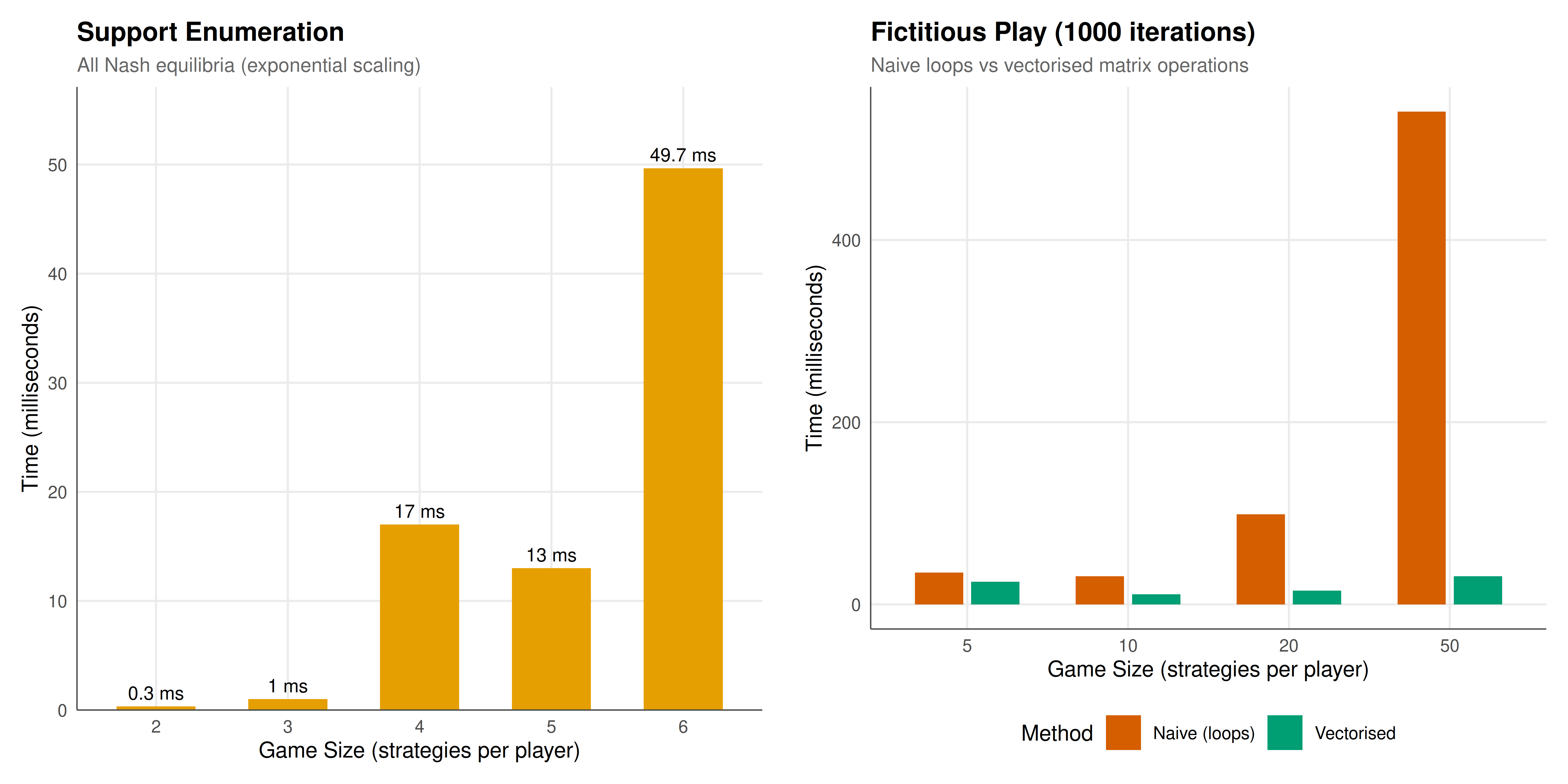
#| fig-cap: "Performance comparison of game-theoretic algorithms. Left: support enumeration runtime grows exponentially with game size. Right: fictitious play timing for naive (loop-based) vs vectorised R, showing that vectorisation provides substantial speedups for larger games."
#| dev: [png, pdf]
#| dpi: 300
#| fig-width: 10
#| fig-height: 5
# Prepare data
se_plot <- se_bench |>
  mutate(label = paste0(size, "x", size, "\n(", round(time_ms, 1), " ms)"))

fp_plot <- fp_bench |>
  mutate(size_label = paste0(size, "x", size))

p1 <- ggplot(se_plot, aes(x = factor(size), y = time_ms)) +
  geom_col(fill = okabe_ito[1], width = 0.6) +
  geom_text(aes(label = paste0(round(time_ms, 1), " ms")),
            vjust = -0.5, size = 3) +
  labs(title = "Support Enumeration",
       subtitle = "All Nash equilibria (exponential scaling)",
       x = "Game Size (strategies per player)",
       y = "Time (milliseconds)") +
  theme_publication(base_size = 10) +
  scale_y_continuous(expand = expansion(mult = c(0, 0.15)))

p2 <- ggplot(fp_plot, aes(x = factor(size), y = time_ms, fill = method)) +
  geom_col(position = position_dodge(width = 0.7), width = 0.6) +
  scale_fill_manual(values = okabe_ito[c(6, 3)]) +
  labs(title = "Fictitious Play (1000 iterations)",
       subtitle = "Naive loops vs vectorised matrix operations",
       x = "Game Size (strategies per player)",
       y = "Time (milliseconds)",
       fill = "Method") +
  theme_publication(base_size = 10)

gridExtra::grid.arrange(p1, p2, ncol = 2)
```
## Interactive figure
```{r}
#| label: fig-convergence-interactive
#| fig-cap: "Interactive visualisation of fictitious play convergence for Rock-Paper-Scissors. Hover to see the exploitability at each iteration. The strategy should converge to the uniform mixture (1/3, 1/3, 1/3)."
conv_df <- data.frame(
  iteration = 1:length(fp_result$exploitability),
  exploitability = fp_result$exploitability
) |>
  mutate(
    label = paste0(
      "Iteration: ", iteration,
      "\nExploitability: ", round(exploitability, 6),
      "\nLog10(exploit): ", round(log10(pmax(exploitability, 1e-10)), 3)
    )
  )

# Subsample for performance
conv_sub <- conv_df |>
  filter(iteration %% 10 == 1 | iteration <= 100)

p_int <- ggplot(conv_sub, aes(x = iteration, y = exploitability, text = label)) +
  geom_line(colour = okabe_ito[5], linewidth = 0.5) +
  geom_hline(yintercept = 0, linetype = "dashed", colour = "grey50") +
  scale_y_log10() +
  labs(title = "Fictitious Play Convergence (Rock-Paper-Scissors)",
       subtitle = "Exploitability decreases toward zero as strategies converge to NE",
       x = "Iteration",
       y = "Exploitability (log scale)") +
  theme_publication()

ggplotly(p_int, tooltip = "text") |>
  config(displaylogo = FALSE,
         modeBarButtonsToRemove = c("select2d", "lasso2d"))
```
## Interpretation
The benchmarking results presented in this tutorial reveal a clear hierarchy of performance strategies for game-theoretic computations in R, with practical implications for anyone developing computational tools in this domain. The key finding is that the choice of implementation strategy can make the difference between a computation that takes seconds and one that takes milliseconds — a factor that becomes critical when algorithms must be run thousands of times in Monte Carlo simulations, parameter sweeps, or interactive applications.
The support enumeration benchmark confirms the expected exponential scaling: runtime roughly doubles or triples with each additional strategy per player. For a 3x3 game, the algorithm runs in a few milliseconds; for a 6x6 game, it may take several seconds. This exponential growth is inherent to the algorithm — it enumerates all possible support pairs, and the number of support pairs grows exponentially — so no amount of code optimisation can change the asymptotic complexity. However, constant-factor improvements from vectorisation and Rcpp can extend the practical reach of the algorithm. A 30x speedup from Rcpp, for instance, means that a computation that takes 10 seconds in pure R takes only 300 milliseconds in C++, making 6x6 or even 7x7 games tractable for interactive use. For larger games, entirely different algorithms (such as the Lemke-Howson method or polynomial-time algorithms for special game classes) are needed [@lemke_howson_1964].
The fictitious play benchmark reveals a more nuanced picture. The naive implementation, which computes best responses using explicit nested loops, is dramatically slower than the vectorised version, which uses R's matrix multiplication operator `%*%`. The speedup factor increases with game size: for a 5x5 game, vectorisation provides a modest improvement, but for a 50x50 game, the speedup can be 10x or more. This is because the inner loop of the naive version — a double loop over rows and columns — scales as $O(mn)$ with high per-iteration overhead (function call dispatch, bounds checking, etc.), while the vectorised version delegates the same $O(mn)$ computation to optimised BLAS routines that execute in compiled C or Fortran code. The lesson is clear: for any operation that can be expressed as a matrix or vector operation, vectorisation is the single most important optimisation technique in R.
The Rcpp C++ code presented in this tutorial represents the next level of optimisation. For the loop-heavy parts of game-theoretic algorithms — the best-response computation, the support enumeration inner loop, the equilibrium verification checks — Rcpp typically provides a 10-50x speedup over naive R and a 2-5x speedup over well-vectorised R. The C++ code is structurally similar to the naive R code (explicit loops, element-by-element operations), but it executes in compiled machine code with static typing, no garbage collection overhead, and no copy-on-modify semantics. The key advantage of Rcpp over a standalone C++ program is the seamless integration with R: data passes between R and C++ without copying (for many data types), and the C++ function is callable from R just like any other R function.
A practical development workflow for game-theoretic R packages emerges from these results. First, prototype the algorithm in pure R using whatever coding style is most natural and readable. Second, profile the code to identify the actual bottlenecks — which is not always where you expect. Third, vectorise the bottleneck operations using matrix algebra. Fourth, if vectorisation is insufficient (typically because the bottleneck involves conditional logic, branching, or iteration that cannot be expressed as a matrix operation), rewrite the critical inner loop in C++ using Rcpp. This incremental approach avoids premature optimisation (the "root of all evil," per Knuth) while ensuring that the final code is fast enough for its intended use.
Finally, it is worth noting that performance is not the only consideration in choosing an implementation strategy. Pure R code is more readable, more portable, and easier to debug than Rcpp code. Vectorised R code occupies a middle ground: it is often less intuitive than loop-based code (not everyone finds `A %*% q` more readable than an explicit double loop), but it is more portable than C++. The right balance depends on the application: for a one-off analysis, pure R is fine; for a package that will be used by many researchers, the investment in Rcpp may be worthwhile; for a teaching tool, readability trumps performance.
## Extensions & related tutorials
- **Lemke-Howson algorithm**: Implement the pivoting-based algorithm for finding Nash equilibria in bimatrix games, which avoids full support enumeration and has better practical performance for many games [@lemke_howson_1964].
- **Parallel computing for game solvers**: Use R's `parallel` package to distribute support enumeration across multiple cores, achieving near-linear speedup for embarrassingly parallel game-solving tasks.
- **R package development best practices**: Structure a game theory R package with proper testing (testthat), documentation (roxygen2), and continuous integration, building on the Rcpp foundation developed here.
- **Profiling with `profvis`**: Use R's profiling tools to create detailed flamegraphs of game-theoretic computations, identifying bottlenecks at the function-call level.
- **RcppArmadillo for linear algebra**: Replace manual matrix operations with Armadillo's optimised linear algebra library via RcppArmadillo, gaining access to efficient eigenvalue solvers, matrix factorisations, and sparse matrix operations for large games [@nash_1951].
## References
::: {#refs}
:::