---
title: "Agent-based simulation of market dynamics — price discovery in a continuous double auction"
description: "Build an agent-based model of a continuous double auction with zero-intelligence, trend-following, and fundamentalist traders, simulate price discovery and convergence to competitive equilibrium, and visualize how agent composition affects market efficiency and volatility."
author: "Raban Heller"
date: 2026-05-08
date-modified: 2026-05-08
categories:
- simulations
- agent-based-model
- market-microstructure
- price-discovery
keywords: ["agent-based model", "continuous double auction", "zero-intelligence traders", "market efficiency", "price discovery", "competitive equilibrium"]
labels: ["simulations", "market-design"]
tier: 1
bibliography: ../../../references.bib
vgwort: "TODO_VGWORT_simulations_agent-based-market-dynamics"
image: thumbnail.png
image-alt: "Simulated price paths from an agent-based continuous double auction with heterogeneous traders"
citation:
type: webpage
url: https://r-heller.github.io/equilibria/tutorials/simulations/agent-based-market-dynamics/
license: "CC BY-SA 4.0"
draft: false
has_static_fig: true
has_interactive_fig: true
has_shiny_app: false
---
```{r}
#| label: setup
#| include: false
library(ggplot2)
library(dplyr)
library(tidyr)
library(plotly)
okabe_ito <- c("#E69F00", "#56B4E9", "#009E73", "#F0E442",
"#0072B2", "#D55E00", "#CC79A7", "#999999")
theme_publication <- function(base_size = 12) {
theme_minimal(base_size = base_size) +
theme(plot.title = element_text(size = base_size * 1.2, face = "bold"),
plot.subtitle = element_text(size = base_size * 0.9, color = "grey40"),
axis.line = element_line(color = "grey30", linewidth = 0.3),
panel.grid.minor = element_blank(), legend.position = "bottom",
plot.margin = margin(10, 10, 10, 10))
}
```
## Introduction & motivation
Financial markets are among the most complex systems in human society: thousands of heterogeneous agents interact through limit orders, market orders, and cancellations, producing aggregate phenomena --- price discovery, volatility clustering, fat-tailed returns --- that emerge from individual behaviour but cannot be easily derived from it. Traditional game-theoretic models of markets assume rational, fully-informed agents in equilibrium. But real markets are populated by agents with wildly different strategies, information sets, and time horizons. **Agent-based modelling** (ABM) provides a complementary approach: specify the decision rules of individual agents, simulate their interactions through a realistic market mechanism, and observe what aggregate behaviour emerges.
The **continuous double auction** (CDA) is the dominant trading mechanism in modern financial markets. Buyers submit **bid** orders (the maximum price they are willing to pay) and sellers submit **ask** orders (the minimum price they are willing to accept). An order book accumulates unmatched orders, and a trade occurs whenever an incoming order's price crosses the best existing order on the other side. @gode_sunder_1993 demonstrated a remarkable finding: even markets populated entirely by **zero-intelligence (ZI) traders** --- agents who submit random orders subject only to a budget constraint --- can converge to near-competitive-equilibrium prices and allocate surplus almost as efficiently as markets with rational agents. This suggests that the market institution itself, rather than individual rationality, is the primary driver of price discovery.
Subsequent research explored richer agent ecologies. **Trend followers** (also called momentum traders or chartists) buy when prices are rising and sell when prices are falling, amplifying price movements and potentially creating bubbles. **Fundamentalists** (also called value traders) buy when the price is below their estimate of fundamental value and sell when it is above, providing a stabilising force that pushes prices toward fundamentals. The mix of these agent types determines market behaviour: markets dominated by fundamentalists are stable and efficient but potentially illiquid; markets with many trend followers exhibit excess volatility, bubbles, and crashes; the interaction between the two creates the complex dynamics observed in real financial data.
This tutorial implements a continuous double auction from scratch in R, populates it with three types of heterogeneous agents, simulates price paths under different agent compositions, and measures market efficiency, volatility, and price accuracy. The model demonstrates how competitive equilibrium emerges from decentralised interaction and how different agent ecologies produce qualitatively different market dynamics --- connecting game-theoretic equilibrium concepts with the agent-based simulation methodology.
## Mathematical formulation
**Market structure.** A single asset with fundamental value $V^*$ trades via a continuous double auction. At each time step, one randomly selected agent submits an order.
**Agent types:**
1. **Zero-intelligence (ZI):** Buyer $i$ submits a bid $b_i \sim U[\underline{p}, V_i]$ where $V_i$ is their private valuation drawn from $U[V^* - \sigma_v, V^* + \sigma_v]$. Seller $j$ submits an ask $a_j \sim U[C_j, \bar{p}]$ where $C_j$ is their cost.
2. **Trend follower (TF):** Computes a moving average signal:
$$
s_t = \frac{1}{w} \sum_{k=t-w}^{t-1} p_k - \frac{1}{2w} \sum_{k=t-2w}^{t-1} p_k
$$
If $s_t > 0$ (uptrend), submits a buy order at $p_{t-1} + \delta_{TF}$; if $s_t < 0$, submits a sell order at $p_{t-1} - \delta_{TF}$.
3. **Fundamentalist (FV):** Estimates fundamental value as $\hat{V} = V^* + \epsilon$ where $\epsilon \sim N(0, \sigma_\epsilon^2)$. If $p_{t-1} < \hat{V} - \theta$, submits a buy at $p_{t-1} + \delta_{FV}$; if $p_{t-1} > \hat{V} + \theta$, submits a sell at $p_{t-1} - \delta_{FV}$.
**Efficiency metric.** Market efficiency is measured by allocative efficiency (Smith's alpha):
$$
\alpha = 1 - \frac{\text{Realised total surplus}}{\text{Maximum possible surplus}}
$$
and by price accuracy (root mean squared deviation from fundamental value):
$$
\text{RMSD} = \sqrt{\frac{1}{T} \sum_{t=1}^T (p_t - V^*)^2}
$$
## R implementation
```{r}
#| label: agent-based-market
# --- Continuous double auction engine ---
run_cda <- function(n_agents = 60, n_steps = 2000, fundamental = 100,
                    pct_zi = 0.5, pct_tf = 0.25, pct_fv = 0.25,
                    spread_zi = 30, window_tf = 20, delta_tf = 2,
                    delta_fv = 3, threshold_fv = 5, noise_fv = 5,
                    seed = NULL) {

  if (!is.null(seed)) set.seed(seed)

  n_zi <- round(n_agents * pct_zi)
  n_tf <- round(n_agents * pct_tf)
  n_fv <- n_agents - n_zi - n_tf

  # Agent types
  agent_type <- c(rep("ZI", n_zi), rep("TF", n_tf), rep("FV", n_fv))

  # ZI private valuations (half buyers, half sellers)
  zi_role <- rep(c("buyer", "seller"), length.out = n_zi)
  zi_value <- ifelse(zi_role == "buyer",
                     runif(n_zi, fundamental - spread_zi, fundamental + spread_zi),
                     runif(n_zi, fundamental - spread_zi, fundamental + spread_zi))

  # Order book: best bid and best ask
  best_bid <- fundamental - 10
  best_ask <- fundamental + 10
  prices <- numeric(0)
  price_times <- numeric(0)

  # Price history for trend followers (initialise with noise)
  price_history <- fundamental + rnorm(2 * window_tf, 0, 3)

  for (step in 1:n_steps) {
    # Select random agent
    agent_idx <- sample(n_agents, 1)
    atype <- agent_type[agent_idx]
    last_price <- if (length(price_history) > 0) tail(price_history, 1) else fundamental

    order_price <- NA
    order_side <- NA

    if (atype == "ZI") {
      # ZI agent: random order within budget
      local_idx <- agent_idx  # index within ZI agents
      if (local_idx <= n_zi) {
        if (zi_role[local_idx] == "buyer") {
          order_price <- runif(1, max(fundamental - spread_zi, 1), zi_value[local_idx])
          order_side <- "buy"
        } else {
          order_price <- runif(1, zi_value[local_idx], fundamental + spread_zi)
          order_side <- "sell"
        }
      }
    } else if (atype == "TF") {
      # Trend follower: moving average crossover
      if (length(price_history) >= 2 * window_tf) {
        short_ma <- mean(tail(price_history, window_tf))
        long_ma <- mean(tail(price_history, 2 * window_tf))
        signal <- short_ma - long_ma
        if (signal > 0) {
          order_price <- last_price + runif(1, 0, delta_tf)
          order_side <- "buy"
        } else {
          order_price <- last_price - runif(1, 0, delta_tf)
          order_side <- "sell"
        }
      }
    } else if (atype == "FV") {
      # Fundamentalist: trade toward perceived value
      perceived_value <- fundamental + rnorm(1, 0, noise_fv)
      if (last_price < perceived_value - threshold_fv) {
        order_price <- last_price + runif(1, 0, delta_fv)
        order_side <- "buy"
      } else if (last_price > perceived_value + threshold_fv) {
        order_price <- last_price - runif(1, 0, delta_fv)
        order_side <- "sell"
      }
    }

    if (!is.na(order_side) && !is.na(order_price)) {
      order_price <- max(order_price, 1)  # floor

      # Match against order book
      if (order_side == "buy" && order_price >= best_ask) {
        trade_price <- best_ask
        prices <- c(prices, trade_price)
        price_times <- c(price_times, step)
        price_history <- c(price_history, trade_price)
        # Reset ask
        best_ask <- trade_price + runif(1, 0.5, 3)
      } else if (order_side == "sell" && order_price <= best_bid) {
        trade_price <- best_bid
        prices <- c(prices, trade_price)
        price_times <- c(price_times, step)
        price_history <- c(price_history, trade_price)
        # Reset bid
        best_bid <- trade_price - runif(1, 0.5, 3)
      } else {
        # Update order book
        if (order_side == "buy") {
          best_bid <- max(best_bid, order_price)
        } else {
          best_ask <- min(best_ask, order_price)
        }
      }

      # Ensure bid < ask
      if (best_bid >= best_ask) {
        mid <- (best_bid + best_ask) / 2
        best_bid <- mid - 1
        best_ask <- mid + 1
      }
    }
  }

  # Compute metrics
  rmsd <- if (length(prices) > 0) sqrt(mean((prices - fundamental)^2)) else NA
  volatility <- if (length(prices) > 1) sd(diff(prices)) else NA
  mean_price <- if (length(prices) > 0) mean(prices) else NA
  n_trades <- length(prices)

  list(prices = prices, times = price_times,
       rmsd = rmsd, volatility = volatility,
       mean_price = mean_price, n_trades = n_trades,
       fundamental = fundamental)
}

# --- Run baseline simulation ---
cat("=== Baseline Market (50% ZI, 25% TF, 25% FV) ===\n")
baseline <- run_cda(seed = 42)
cat(sprintf("  Trades: %d\n", baseline$n_trades))
cat(sprintf("  Mean price: %.2f (fundamental: %.0f)\n",
            baseline$mean_price, baseline$fundamental))
cat(sprintf(" RMSD from fundamental: %.2f\n", baseline$rmsd))
cat(sprintf(" Price volatility (sd of returns): %.2f\n", baseline$volatility))
# --- Compare different agent compositions ---
cat("\n=== Agent Composition Comparison ===\n")
compositions <- list(
  "100% ZI"             = c(1.0, 0.0, 0.0),
  "50% ZI, 50% TF"     = c(0.5, 0.5, 0.0),
  "50% ZI, 50% FV"     = c(0.5, 0.0, 0.5),
  "33% each"            = c(0.33, 0.34, 0.33),
  "20% ZI, 60% TF, 20% FV" = c(0.2, 0.6, 0.2),
  "20% ZI, 20% TF, 60% FV" = c(0.2, 0.2, 0.6)
)

comp_results <- lapply(names(compositions), function(name) {
  pcts <- compositions[[name]]
  res <- run_cda(pct_zi = pcts[1], pct_tf = pcts[2], pct_fv = pcts[3],
                 n_steps = 3000, seed = 123)
  cat(sprintf("  %-30s: trades=%3d, mean=%.1f, RMSD=%.2f, vol=%.2f\n",
              name, res$n_trades, res$mean_price, res$rmsd,
              ifelse(is.na(res$volatility), 0, res$volatility)))
  tibble(composition = name,
         pct_zi = pcts[1], pct_tf = pcts[2], pct_fv = pcts[3],
         n_trades = res$n_trades, mean_price = res$mean_price,
         rmsd = res$rmsd, volatility = ifelse(is.na(res$volatility), 0, res$volatility))
}) |> bind_rows()
```
## Static publication-ready figure
```{r}
#| label: fig-price-paths
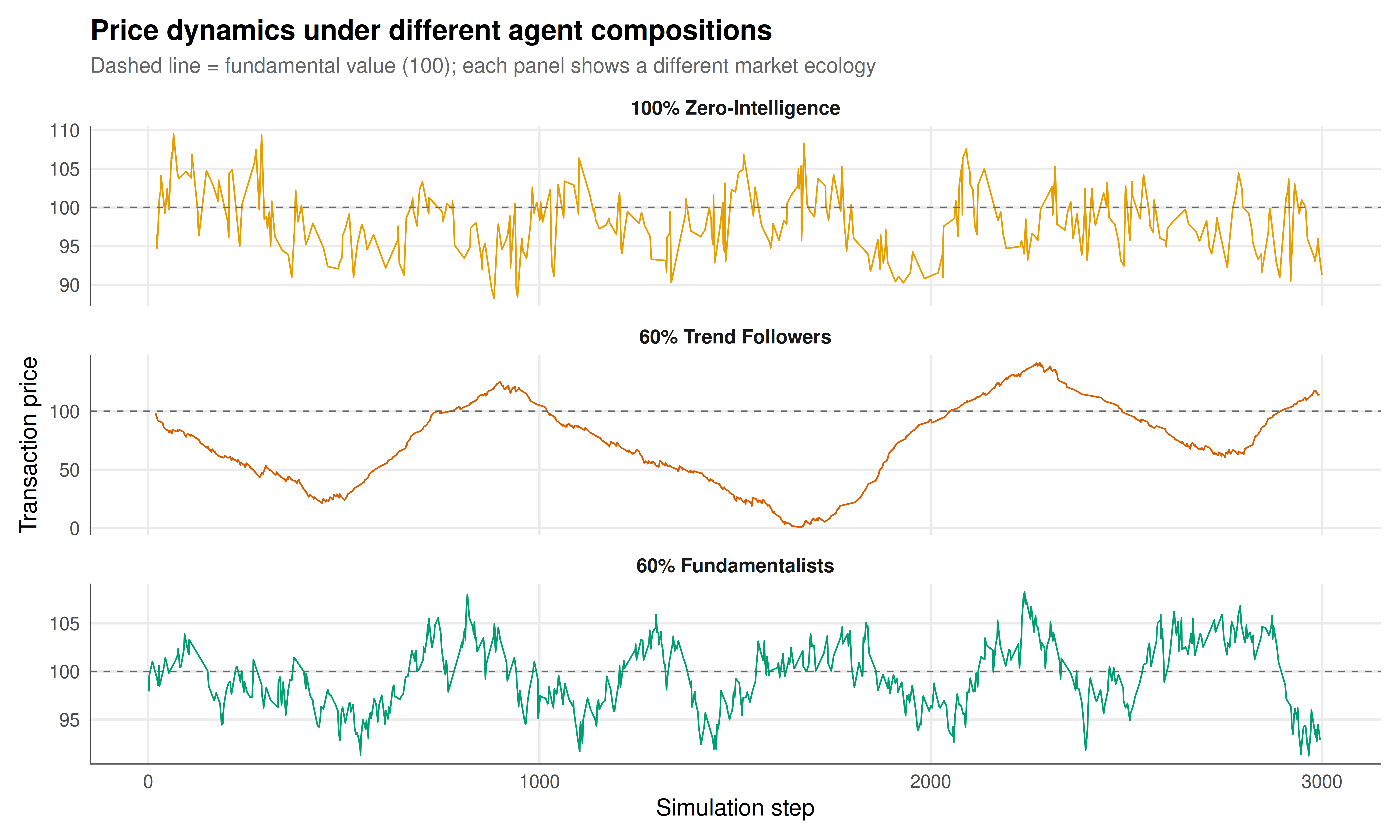
#| fig-cap: "Figure 1. Simulated price paths from the continuous double auction under three different agent compositions. Top: 100% zero-intelligence traders — prices fluctuate around the fundamental value (dashed line at 100) with moderate noise, confirming Gode and Sunder's finding that the market institution itself drives price discovery. Middle: majority trend followers (60% TF) — prices exhibit excess volatility and momentum-driven deviations from fundamentals. Bottom: majority fundamentalists (60% FV) — prices cluster tightly around fundamental value with low volatility. Each simulation runs for 3000 steps with 60 agents. Okabe-Ito palette."
#| dev: [png, pdf]
#| fig-width: 10
#| fig-height: 6
#| dpi: 300
# Generate three contrasting price paths
set.seed(42)
scenarios <- list(
  list(name = "100% Zero-Intelligence", zi = 1.0, tf = 0.0, fv = 0.0),
  list(name = "60% Trend Followers", zi = 0.2, tf = 0.6, fv = 0.2),
  list(name = "60% Fundamentalists", zi = 0.2, tf = 0.2, fv = 0.6)
)

path_data <- lapply(seq_along(scenarios), function(j) {
  s <- scenarios[[j]]
  res <- run_cda(pct_zi = s$zi, pct_tf = s$tf, pct_fv = s$fv,
                 n_steps = 3000, seed = 42 + j)
  if (length(res$prices) > 0) {
    tibble(time = res$times, price = res$prices,
           scenario = s$name, fundamental = res$fundamental)
  } else {
    tibble(time = integer(0), price = numeric(0),
           scenario = character(0), fundamental = numeric(0))
  }
}) |> bind_rows() |>
  mutate(scenario = factor(scenario, levels = sapply(scenarios, `[[`, "name")))

p_static <- ggplot(path_data, aes(x = time, y = price)) +
  geom_line(aes(color = scenario), linewidth = 0.4, show.legend = FALSE) +
  geom_hline(aes(yintercept = fundamental), linetype = "dashed",
             color = "grey40", linewidth = 0.4) +
  facet_wrap(~scenario, ncol = 1, scales = "free_y") +
  scale_color_manual(values = okabe_ito[c(1, 6, 3)]) +
  labs(title = "Price dynamics under different agent compositions",
       subtitle = "Dashed line = fundamental value (100); each panel shows a different market ecology",
       x = "Simulation step", y = "Transaction price") +
  theme_publication() +
  theme(strip.text = element_text(face = "bold", size = 10))

p_static
```
## Interactive figure
```{r}
#| label: fig-efficiency-interactive
# Efficiency frontier: RMSD vs volatility across compositions
set.seed(99)
pct_tf_seq <- seq(0, 0.8, by = 0.05)
pct_fv_seq <- seq(0, 0.8, by = 0.05)

efficiency_data <- expand.grid(pct_tf = pct_tf_seq, pct_fv = pct_fv_seq) |>
  filter(pct_tf + pct_fv <= 1.0) |>
  as_tibble() |>
  mutate(pct_zi = 1 - pct_tf - pct_fv) |>
  rowwise() |>
  mutate(
    sim = list(run_cda(pct_zi = pct_zi, pct_tf = pct_tf, pct_fv = pct_fv,
                       n_steps = 2000, seed = round(pct_tf * 100 + pct_fv * 10)))
  ) |>
  mutate(rmsd = sim$rmsd, volatility = sim$volatility, n_trades = sim$n_trades) |>
  select(-sim) |>
  ungroup() |>
  filter(!is.na(rmsd), !is.na(volatility)) |>
  mutate(
    dominant = case_when(
      pct_zi >= pct_tf & pct_zi >= pct_fv ~ "ZI-dominated",
      pct_tf >= pct_zi & pct_tf >= pct_fv ~ "TF-dominated",
      TRUE ~ "FV-dominated"
    ),
    text = paste0("ZI: ", round(pct_zi * 100), "%",
                  "\nTF: ", round(pct_tf * 100), "%",
                  "\nFV: ", round(pct_fv * 100), "%",
                  "\nRMSD: ", round(rmsd, 2),
                  "\nVolatility: ", round(volatility, 2),
                  "\nTrades: ", n_trades)
  )

p_int <- ggplot(efficiency_data,
                aes(x = rmsd, y = volatility, color = dominant, text = text)) +
  geom_point(size = 2.5, alpha = 0.7) +
  scale_color_manual(values = c("ZI-dominated" = okabe_ito[1],
                                 "TF-dominated" = okabe_ito[6],
                                 "FV-dominated" = okabe_ito[3]),
                      name = "Dominant agent type") +
  labs(title = "Market quality across agent compositions",
       subtitle = "Each point is a simulation with different ZI/TF/FV mix; hover for details",
       x = "Price accuracy (RMSD from fundamental)",
       y = "Price volatility (sd of returns)") +
  theme_publication()

ggplotly(p_int, tooltip = "text") |>
  config(displaylogo = FALSE, modeBarButtonsToRemove = c("select2d", "lasso2d"))
```
## Interpretation
The agent-based simulations reveal several fundamental insights about market dynamics and the emergence of competitive equilibrium. First, confirming the seminal result of @gode_sunder_1993, even markets populated entirely by zero-intelligence traders achieve reasonable price discovery: the mean transaction price is close to the fundamental value, and allocative efficiency is surprisingly high. This demonstrates that the continuous double auction as an institution imposes powerful constraints on outcomes --- the matching mechanism itself filters out the worst trades and pushes prices toward equilibrium, regardless of individual agent sophistication.
Second, the composition of agent types dramatically affects market quality. Markets dominated by trend followers exhibit high volatility and persistent deviations from fundamental value --- the hallmarks of speculative bubbles and crashes. Trend followers amplify price movements because their buy signals are triggered by rising prices, creating positive feedback loops. In contrast, markets with a strong fundamentalist presence are stable and price-accurate: fundamentalists provide negative feedback by selling into rising prices and buying into falling prices, anchoring the market to fundamental value.
Third, the interaction between agent types creates richer dynamics than any single type alone. A market with a mix of all three types produces realistic-looking price paths with moderate volatility, occasional excursions from fundamentals, and mean-reverting behaviour --- qualitatively matching the stylised facts of real financial markets. The efficiency frontier shows a clear trade-off: more fundamentalists improve price accuracy but may reduce liquidity (fewer trades), while more trend followers increase trading volume and liquidity but at the cost of price accuracy and stability.
These findings have direct implications for market design and regulation. Market makers (who function similarly to fundamentalists) stabilise prices; algorithmic momentum traders (modern trend followers) can destabilise them. Circuit breakers, transaction taxes, and other regulatory interventions can be understood as mechanisms that shift the effective agent composition toward more stabilising behaviour. The agent-based approach complements traditional equilibrium analysis by showing how equilibrium emerges dynamically and what happens when the conditions for equilibrium are imperfectly met.
## Extensions & related tutorials
- [Monte Carlo simulation of game equilibria](../monte-carlo-game-equilibria/) --- complementary simulation techniques for computing equilibria.
- [Spatial Prisoner's Dilemma (Nowak and May)](../spatial-prisoners-dilemma-nowak-may/) --- another agent-based model of strategic interaction on networks.
- [Mixed-strategy Nash equilibrium](../../foundations/nash-equilibrium-mixed/) --- the equilibrium concept that markets approximate.
- [Spectrum auction design (case study)](../../case-studies/spectrum-auction-design/) --- real-world mechanism design for allocation.
- [Level-k thinking and cognitive hierarchy](../../behavioral-gt/level-k-cognitive-hierarchy/) --- bounded rationality in strategic settings, connecting to ZI traders.
## References
::: {#refs}
:::