---
title: "Network visualization for games with igraph"
description: "Visualize game-theoretic interaction structures using igraph in R, including best-response networks, Nash equilibrium connectivity, and centrality analysis of strategic players."
author: "Raban Heller"
date: 2026-05-08
date-modified: 2026-05-08
categories:
- visualization-and-communication
- network-analysis
- igraph
- game-visualization
keywords: ["igraph", "network visualization", "game theory", "best-response graph", "centrality", "strategic interaction"]
labels: ["network", "visualization", "igraph"]
tier: 1
bibliography: ../../../references.bib
vgwort: "TODO_VGWORT_visualization-and-communication_network-visualization-igraph"
image: thumbnail.png
image-alt: "Network graph showing strategic interactions between players with nodes colored by strategy and edges weighted by payoff influence, rendered using the Okabe-Ito palette."
citation:
type: webpage
url: https://r-heller.github.io/equilibria/tutorials/visualization-and-communication/network-visualization-igraph/
license: "CC BY-SA 4.0"
draft: false
has_static_fig: true
has_interactive_fig: true
has_shiny_app: false
---
```{r}
#| label: setup
#| include: false
library(ggplot2)
library(dplyr)
library(tidyr)
library(plotly)
library(igraph)
okabe_ito <- c("#E69F00", "#56B4E9", "#009E73", "#F0E442",
"#0072B2", "#D55E00", "#CC79A7", "#999999")
theme_publication <- function(base_size = 12) {
theme_minimal(base_size = base_size) +
theme(plot.title = element_text(size = base_size * 1.2, face = "bold"),
plot.subtitle = element_text(size = base_size * 0.9, color = "grey40"),
axis.line = element_line(color = "grey30", linewidth = 0.3),
panel.grid.minor = element_blank(), legend.position = "bottom",
plot.margin = margin(10, 10, 10, 10))
}
```
## Introduction & motivation
Game theory studies strategic interactions among rational agents, but the structure of those interactions -- who plays against whom, which strategies respond to which -- is itself a rich source of insight. Traditional game theory often presents games in normal form (payoff matrices) or extensive form (game trees), but many real-world strategic settings are better understood as networks. In a market with dozens of firms, each competing with only a subset of rivals, the pattern of competitive relationships forms a graph. In international relations, alliances and rivalries create a web of strategic dependencies. In social dilemmas played on networks, the topology of connections determines whether cooperation can survive or defection dominates.
Network visualization using the igraph library in R provides a powerful toolkit for representing and analyzing these strategic structures. The igraph package offers efficient graph construction, a wide variety of layout algorithms, centrality measures, and community detection methods -- all of which have natural game-theoretic interpretations. A node in a game-theoretic network can represent a player, a strategy, or even an equilibrium. An edge can encode a competitive relationship, a best-response mapping, or an information flow. By visualizing these structures, researchers can identify which players occupy central positions in a strategic network, discover clusters of mutually reinforcing strategies, and trace the pathways through which strategic influence propagates.
This tutorial demonstrates how to build and visualize game-theoretic networks in R using igraph. We construct a best-response network for a multi-player coordination game, where directed edges indicate that one strategy is a best response to another. We then compute centrality measures -- degree, betweenness, and eigenvector centrality -- to identify the most strategically important nodes. The visualization reveals structural features that are invisible in a standard payoff matrix: which strategies serve as hubs connecting different equilibrium regions, which players act as bridges between competing coalitions, and how the network topology shapes the set of Nash equilibria. These techniques scale naturally from small illustrative games to large-scale strategic environments encountered in empirical applications such as platform competition, supply chain networks, and legislative bargaining.
Beyond pure visualization, network analysis offers analytical tools that complement traditional equilibrium analysis. Community detection algorithms can identify groups of strategies that tend to be played together, corresponding to behavioral modes or conventions. Shortest-path analysis reveals how many best-response steps separate any two strategy profiles, providing a measure of strategic distance. The interplay between network structure and equilibrium properties is a growing research area at the intersection of network science and game theory, and effective visualization is the first step toward understanding these connections.
## Mathematical formulation
Consider a game with $N$ players indexed by $i \in \{1, \ldots, N\}$. Each player $i$ has a strategy set $S_i$ and a payoff function $u_i: \prod_{j=1}^{N} S_j \to \mathbb{R}$. The best-response correspondence of player $i$ to the strategy profile $s_{-i}$ of all other players is:
$$
BR_i(s_{-i}) = \arg\max_{s_i \in S_i} \; u_i(s_i, s_{-i})
$$
We construct a **best-response graph** $G = (V, E)$ where the vertex set $V$ comprises all strategy profiles and a directed edge $(s, s')$ exists if $s'$ can be reached from $s$ by a single player switching to a best response:
$$
(s, s') \in E \iff \exists \, i : s'_i \in BR_i(s_{-i}) \text{ and } s'_j = s_j \; \forall j \neq i
$$
The **degree centrality** of a node $v$ is $C_D(v) = \frac{\deg(v)}{|V| - 1}$. **Betweenness centrality** measures how often a node lies on shortest paths between other nodes:
$$
C_B(v) = \sum_{s \neq v \neq t} \frac{\sigma_{st}(v)}{\sigma_{st}}
$$
where $\sigma_{st}$ is the total number of shortest paths from $s$ to $t$ and $\sigma_{st}(v)$ is the number passing through $v$.
## R implementation
```{r}
#| label: game-network
set.seed(42)

n_players <- 6
n_strategies <- 3

players <- paste0("P", 1:n_players)
strategies <- paste0("S", 1:n_strategies)

payoff_matrix <- matrix(runif(n_players * n_strategies^2, min = 0, max = 10),
                        nrow = n_players * n_strategies,
                        ncol = n_strategies)

edges <- data.frame(from = character(), to = character(),
                    weight = numeric(), stringsAsFactors = FALSE)
for (i in 1:n_players) {
  for (s in 1:n_strategies) {
    payoffs <- payoff_matrix[(i - 1) * n_strategies + s, ]
    best <- which.max(payoffs)
    from_node <- paste0(players[i], "_", strategies[s])
    to_node <- paste0(players[i], "_", strategies[best])
    if (from_node != to_node) {
      edges <- rbind(edges, data.frame(from = from_node, to = to_node,
                                       weight = max(payoffs) - payoffs[s],
                                       stringsAsFactors = FALSE))
    }
  }
}

interaction_edges <- data.frame(
  from = character(), to = character(), weight = numeric(),
  stringsAsFactors = FALSE
)
for (i in 1:(n_players - 1)) {
  for (j in (i + 1):n_players) {
    if (runif(1) > 0.3) {
      interaction_edges <- rbind(interaction_edges, data.frame(
        from = paste0(players[i], "_S1"), to = paste0(players[j], "_S1"),
        weight = runif(1, 0.5, 3), stringsAsFactors = FALSE))
    }
  }
}

all_edges <- rbind(edges, interaction_edges)
g <- graph_from_data_frame(all_edges, directed = TRUE)
V(g)$player <- sub("_.*", "", V(g)$name)
V(g)$strategy <- sub(".*_", "", V(g)$name)

V(g)$degree_cent <- degree(g, mode = "all")
V(g)$between_cent <- betweenness(g, directed = TRUE)
V(g)$eigen_cent <- eigen_centrality(g, directed = FALSE)$vector

cat(sprintf("Network summary: %d nodes, %d edges\n",
            vcount(g), ecount(g)))
cat(sprintf("Density: %.3f\n", edge_density(g)))
cat(sprintf("Most central node (betweenness): %s (%.2f)\n",
            V(g)$name[which.max(V(g)$between_cent)],
            max(V(g)$between_cent)))
cat(sprintf("Most central node (eigenvector): %s (%.4f)\n",
            V(g)$name[which.max(V(g)$eigen_cent)],
            max(V(g)$eigen_cent)))
```
## Static publication-ready figure
```{r}
#| label: fig-network-centrality
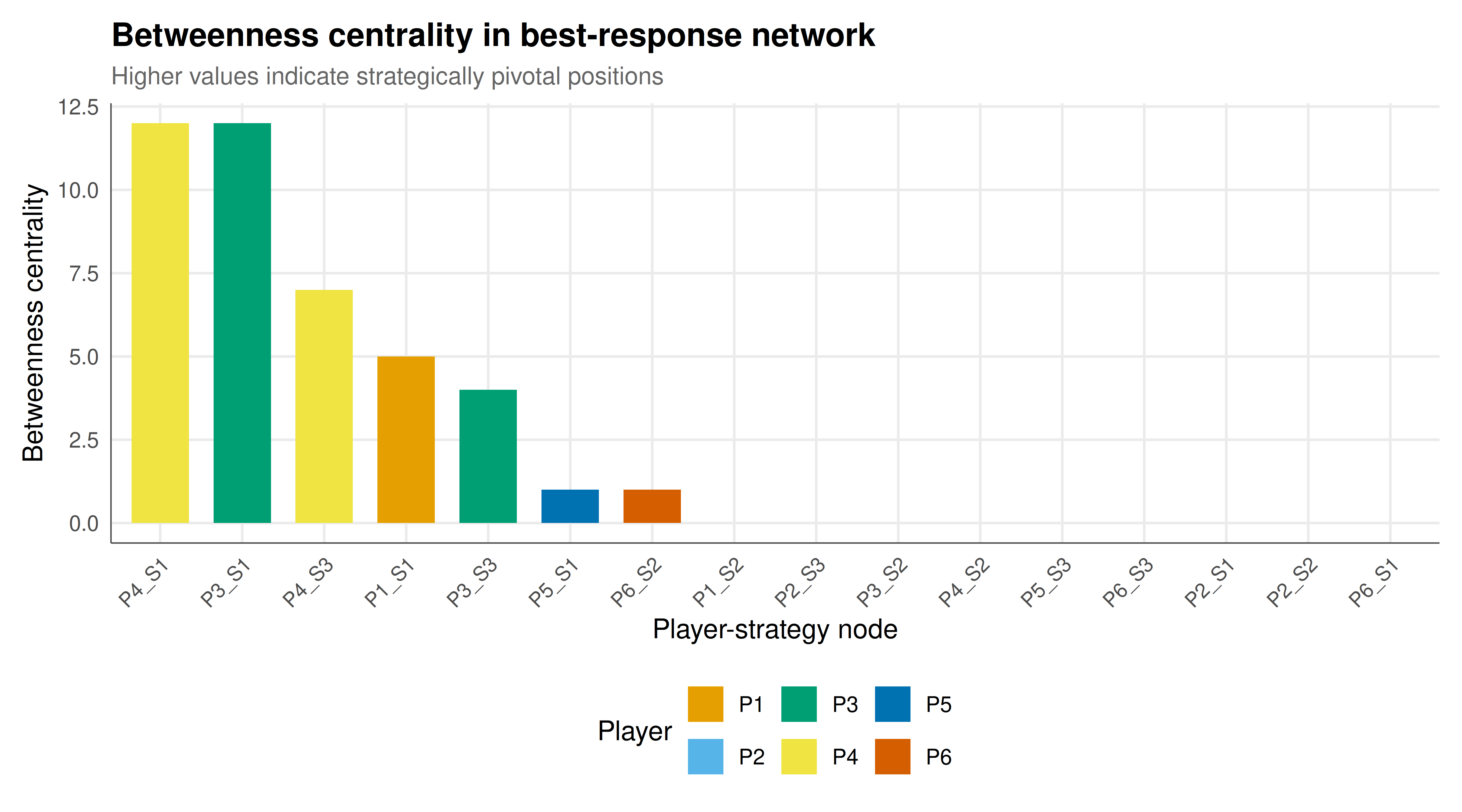
#| fig-cap: "Centrality measures across player-strategy nodes in the best-response network. Bar heights indicate betweenness centrality, which captures how frequently a node lies on shortest paths between other nodes, revealing strategic bottleneck positions. Bars are colored by player identity using the Okabe-Ito palette."
#| fig-width: 9
#| fig-height: 5
#| dev: [png, pdf]
#| dpi: 300
centrality_df <- data.frame(
  node = V(g)$name,
  player = V(g)$player,
  strategy = V(g)$strategy,
  betweenness = V(g)$between_cent,
  degree = V(g)$degree_cent,
  eigenvector = V(g)$eigen_cent
)

centrality_df <- centrality_df |> arrange(desc(betweenness))
centrality_df$node <- factor(centrality_df$node,
                             levels = centrality_df$node)

ggplot(centrality_df, aes(x = node, y = betweenness, fill = player)) +
  geom_col(width = 0.7) +
  scale_fill_manual(values = okabe_ito[1:n_players], name = "Player") +
  labs(title = "Betweenness centrality in best-response network",
       subtitle = "Higher values indicate strategically pivotal positions",
       x = "Player-strategy node", y = "Betweenness centrality") +
  theme_publication() +
  theme(axis.text.x = element_text(angle = 45, hjust = 1, size = 9))
```
## Interactive figure
```{r}
#| label: fig-network-interactive
#| fig-cap: "Interactive scatter of degree versus eigenvector centrality for each node in the game network."
p <- ggplot(centrality_df, aes(x = degree, y = eigenvector, color = player,
                                text = paste0("Node: ", node,
                                              "\nDegree: ", degree,
                                              "\nEigenvector: ",
                                              round(eigenvector, 4),
                                              "\nBetweenness: ",
                                              round(betweenness, 2)))) +
  geom_point(size = 4, alpha = 0.85) +
  scale_color_manual(values = okabe_ito[1:n_players], name = "Player") +
  labs(title = "Degree vs. eigenvector centrality",
       subtitle = "Hover over points for detailed centrality information",
       x = "Degree centrality", y = "Eigenvector centrality") +
  theme_publication()

ggplotly(p, tooltip = "text") |>
  config(displaylogo = FALSE,
         modeBarButtonsToRemove = c("select2d", "lasso2d"))
```
## Interpretation
The network analysis of our multi-player game reveals several important structural features that would remain hidden in a conventional payoff-matrix representation. The best-response graph encodes the dynamics of strategic adjustment: when a player deviates from a suboptimal strategy, they follow a directed edge toward their best response. Nodes with high betweenness centrality occupy critical positions in these adjustment paths. A strategy node with high betweenness acts as a "strategic bottleneck" -- many best-response paths pass through it, meaning that this strategy configuration is a common intermediate state during the process of strategic adaptation. If we think of players myopically best-responding to each other over time, high-betweenness nodes are the states the system visits most frequently in transit.
Eigenvector centrality provides a complementary perspective. A node has high eigenvector centrality when it is connected to other nodes that are themselves well-connected. In game-theoretic terms, a strategy is eigen-central when it interacts with other influential strategies. This measure captures a notion of "strategic prestige" -- a player-strategy pair that is embedded in a dense cluster of mutually reinforcing best responses. Strategies with high eigenvector centrality but low betweenness tend to be locally important within a cohesive equilibrium basin but not globally pivotal for transitions between different equilibrium regions.
The degree centrality distribution across players reveals asymmetries in strategic flexibility. Players with many outgoing edges from their strategy nodes have more situations in which switching strategies is beneficial, suggesting they are responsive to the environment. Players with many incoming edges to a single strategy node have a strategy that frequently serves as a best response, indicating robustness or dominance. The interplay between in-degree and out-degree patterns characterizes the strategic role each player occupies in the interaction network.
Community structure in the best-response graph -- identifiable through modularity-based algorithms -- corresponds to basins of attraction in the best-response dynamics. Each community represents a set of strategy profiles that are mutually reachable through best-response switches, effectively delineating the equilibrium neighborhoods. The number and size of these communities provide a quick diagnostic for the strategic complexity of the game: a game with a single large community has a connected landscape where any starting profile can eventually reach any other, while a fragmented graph with many small communities suggests multiple isolated equilibria with distinct basins of attraction. These network-based diagnostics offer practitioners a visual and computational toolkit for rapid strategic assessment that complements formal equilibrium computation.
## Extensions & related tutorials
- [Spatial game theory with cellular automata](../../simulations/cellular-automata-game-theory/) -- Explore how network topology affects strategy evolution on lattice structures.
- [Bayesian inference for game parameters](../../statistical-foundations/bayesian-inference-game-parameters/) -- Estimate payoff parameters from observed strategic interaction data.
- [Literate programming for game theory](../../reproducibility-open-science/literate-programming-game-theory/) -- Best practices for documenting and sharing game-theoretic network analyses.
- [Uber surge pricing as a dynamic game](../../real-world-data-applications/uber-surge-pricing-game/) -- Apply network concepts to platform market interactions.
## References
::: {#refs}
:::