---
title: "Bayesian inference for game-theoretic parameters"
description: "Estimate game parameters including payoffs, type distributions, and rationality levels from observed play using Bayesian methods with quantal response equilibrium likelihoods and grid-based posterior computation."
author: "Raban Heller"
date: 2026-05-08
date-modified: 2026-05-08
categories:
- statistical-foundations
- bayesian-inference
- qre
- parameter-estimation
keywords: ["Bayesian inference", "game theory", "quantal response equilibrium", "posterior distribution", "likelihood", "logit choice", "grid approximation"]
labels: ["bayesian", "estimation", "qre"]
tier: 1
bibliography: ../../../references.bib
vgwort: "TODO_VGWORT_statistical-foundations_bayesian-inference-game-parameters"
image: thumbnail.png
image-alt: "Posterior density plot showing the Bayesian estimate of a rationality parameter lambda from observed game play data, with prior and posterior distributions overlaid using the Okabe-Ito palette."
citation:
type: webpage
url: https://r-heller.github.io/equilibria/tutorials/statistical-foundations/bayesian-inference-game-parameters/
license: "CC BY-SA 4.0"
draft: false
has_static_fig: true
has_interactive_fig: true
has_shiny_app: false
---
```{r}
#| label: setup
#| include: false
library(ggplot2)
library(dplyr)
library(tidyr)
library(plotly)
okabe_ito <- c("#E69F00", "#56B4E9", "#009E73", "#F0E442",
"#0072B2", "#D55E00", "#CC79A7", "#999999")
theme_publication <- function(base_size = 12) {
theme_minimal(base_size = base_size) +
theme(plot.title = element_text(size = base_size * 1.2, face = "bold"),
plot.subtitle = element_text(size = base_size * 0.9, color = "grey40"),
axis.line = element_line(color = "grey30", linewidth = 0.3),
panel.grid.minor = element_blank(), legend.position = "bottom",
plot.margin = margin(10, 10, 10, 10))
}
```
## Introduction & motivation
A persistent challenge in empirical game theory is bridging the gap between theoretical models and observed behavior. Game-theoretic models predict that players will choose strategies according to equilibrium concepts -- Nash equilibrium, dominant strategy equilibrium, or refinements thereof -- but real human players deviate from these predictions in systematic ways. They make errors, have heterogeneous beliefs, and may not fully optimize. The quantal response equilibrium (QRE) framework, introduced by McKelvey and Palfrey (1995), addresses this by modeling players as choosing strategies with probabilities that increase in expected payoffs but allow for stochastic deviations. The key parameter governing the degree of rationality is the precision parameter $\lambda$: when $\lambda = 0$, players choose uniformly at random; as $\lambda \to \infty$, play converges to Nash equilibrium.
Bayesian inference provides a principled framework for estimating $\lambda$ and other game parameters from experimental or observational data. Unlike frequentist point estimation, the Bayesian approach yields a full posterior distribution over the parameter space, quantifying uncertainty in a way that is especially valuable when sample sizes are small -- as they often are in laboratory experiments. The posterior distribution also incorporates prior information, which is useful when previous experiments or theoretical considerations suggest plausible parameter ranges. For instance, a meta-analysis of experimental games might establish that $\lambda$ typically falls between 1 and 10 for most subject populations, and this knowledge can be encoded in an informative prior.
This tutorial implements Bayesian estimation of the QRE rationality parameter from simulated experimental data. We consider a symmetric two-player game with three strategies, generate observed choice frequencies from a QRE with known $\lambda$, and then recover $\lambda$ using grid-based posterior computation. The grid approximation approach is transparent, requires no specialized MCMC software, and provides exact results (up to grid resolution). For each candidate value of $\lambda$ on a fine grid, we compute the QRE choice probabilities, evaluate the multinomial likelihood of the observed data, multiply by the prior, and normalize to obtain the posterior. This workflow illustrates the core logic of Bayesian inference without the complexity of sampling algorithms, making it accessible to researchers with standard R skills.
The Bayesian perspective is particularly natural for game theory because games inherently involve beliefs. A player's strategy choice depends on beliefs about the opponent's strategy, which in turn depends on beliefs about the opponent's beliefs, and so on. Bayesian inference extends this epistemic hierarchy to the analyst: the researcher holds beliefs (the prior) about the parameters governing player behavior, observes data (strategy choices), and updates beliefs to form the posterior. The coherence of this framework -- beliefs about beliefs, updated through evidence -- makes Bayesian methods a philosophically and practically appropriate tool for empirical game theory. Moreover, the posterior distribution directly answers the decision-relevant questions: what parameter values are consistent with the data, how precisely are they identified, and how does uncertainty about parameters translate into uncertainty about equilibrium predictions.
## Mathematical formulation
Consider a symmetric two-player game with strategy set $S = \{1, 2, 3\}$ and payoff matrix $A = [a_{ij}]$. In a logit QRE, each player chooses strategy $j$ with probability:
$$
\sigma_j(\lambda) = \frac{\exp(\lambda \cdot \mathbb{E}[u_j])}{\sum_{k \in S} \exp(\lambda \cdot \mathbb{E}[u_k])}
$$
where $\mathbb{E}[u_j] = \sum_k a_{jk} \, \sigma_k(\lambda)$ is the expected payoff from strategy $j$ given the opponent plays according to $\sigma(\lambda)$. This defines a fixed-point equation $\sigma = QRE(\lambda, \sigma)$.
Given observed strategy counts $n = (n_1, n_2, n_3)$ from $N = \sum_j n_j$ independent observations, the **likelihood** is multinomial:
$$
L(\lambda \mid n) = \binom{N}{n_1, n_2, n_3} \prod_{j=1}^{3} \sigma_j(\lambda)^{n_j}
$$
With prior $\pi(\lambda)$, the **posterior** is:
$$
p(\lambda \mid n) = \frac{L(\lambda \mid n) \, \pi(\lambda)}{\int_0^{\Lambda} L(\lambda' \mid n) \, \pi(\lambda') \, d\lambda'}
$$
## R implementation
```{r}
#| label: bayesian-qre
set.seed(42)

payoff_matrix <- matrix(c(
  3, 0, 5,
  5, 3, 0,
  0, 5, 3
), nrow = 3, byrow = TRUE)

compute_qre <- function(lambda, A, tol = 1e-8, max_iter = 1000) {
  n_strategies <- nrow(A)
  sigma <- rep(1 / n_strategies, n_strategies)
  for (iter in 1:max_iter) {
    expected_payoffs <- A %*% sigma
    log_probs <- lambda * as.numeric(expected_payoffs)
    log_probs <- log_probs - max(log_probs)
    sigma_new <- exp(log_probs) / sum(exp(log_probs))
    if (max(abs(sigma_new - sigma)) < tol) break
    sigma <- sigma_new
  }
  return(as.numeric(sigma_new))
}

lambda_true <- 2.5
n_obs <- 120

qre_probs <- compute_qre(lambda_true, payoff_matrix)
observed_counts <- as.numeric(rmultinom(1, n_obs, qre_probs))
cat(sprintf("True lambda: %.2f\n", lambda_true))
cat(sprintf("QRE probabilities: [%.4f, %.4f, %.4f]\n",
            qre_probs[1], qre_probs[2], qre_probs[3]))
cat(sprintf("Observed counts: [%d, %d, %d] (N = %d)\n",
            observed_counts[1], observed_counts[2], observed_counts[3], n_obs))
lambda_grid <- seq(0.01, 10, length.out = 500)
prior <- dgamma(lambda_grid, shape = 2, rate = 0.5)
prior <- prior / sum(prior)

log_likelihood <- numeric(length(lambda_grid))
for (i in seq_along(lambda_grid)) {
  probs_i <- compute_qre(lambda_grid[i], payoff_matrix)
  probs_i <- pmax(probs_i, 1e-15)
  log_likelihood[i] <- sum(observed_counts * log(probs_i))
}

log_posterior_unnorm <- log_likelihood + log(prior)
log_posterior_unnorm <- log_posterior_unnorm - max(log_posterior_unnorm)
posterior <- exp(log_posterior_unnorm)
posterior <- posterior / sum(posterior)

map_idx <- which.max(posterior)
lambda_map <- lambda_grid[map_idx]
post_mean <- sum(lambda_grid * posterior)
post_var <- sum((lambda_grid - post_mean)^2 * posterior)

cdf <- cumsum(posterior)
ci_low <- lambda_grid[min(which(cdf >= 0.025))]
ci_high <- lambda_grid[min(which(cdf >= 0.975))]

cat(sprintf("\nPosterior summary:\n"))
cat(sprintf(" MAP estimate: %.3f\n", lambda_map))
cat(sprintf(" Posterior mean: %.3f\n", post_mean))
cat(sprintf(" Posterior SD: %.3f\n", sqrt(post_var)))
cat(sprintf(" 95%% credible interval: [%.3f, %.3f]\n", ci_low, ci_high))
posterior_df <- data.frame(
  lambda = lambda_grid,
  prior = prior / max(prior),
  posterior = posterior / max(posterior),
  likelihood = exp(log_likelihood - max(log_likelihood))
)
```
## Static publication-ready figure
```{r}
#| label: fig-bayesian-posterior
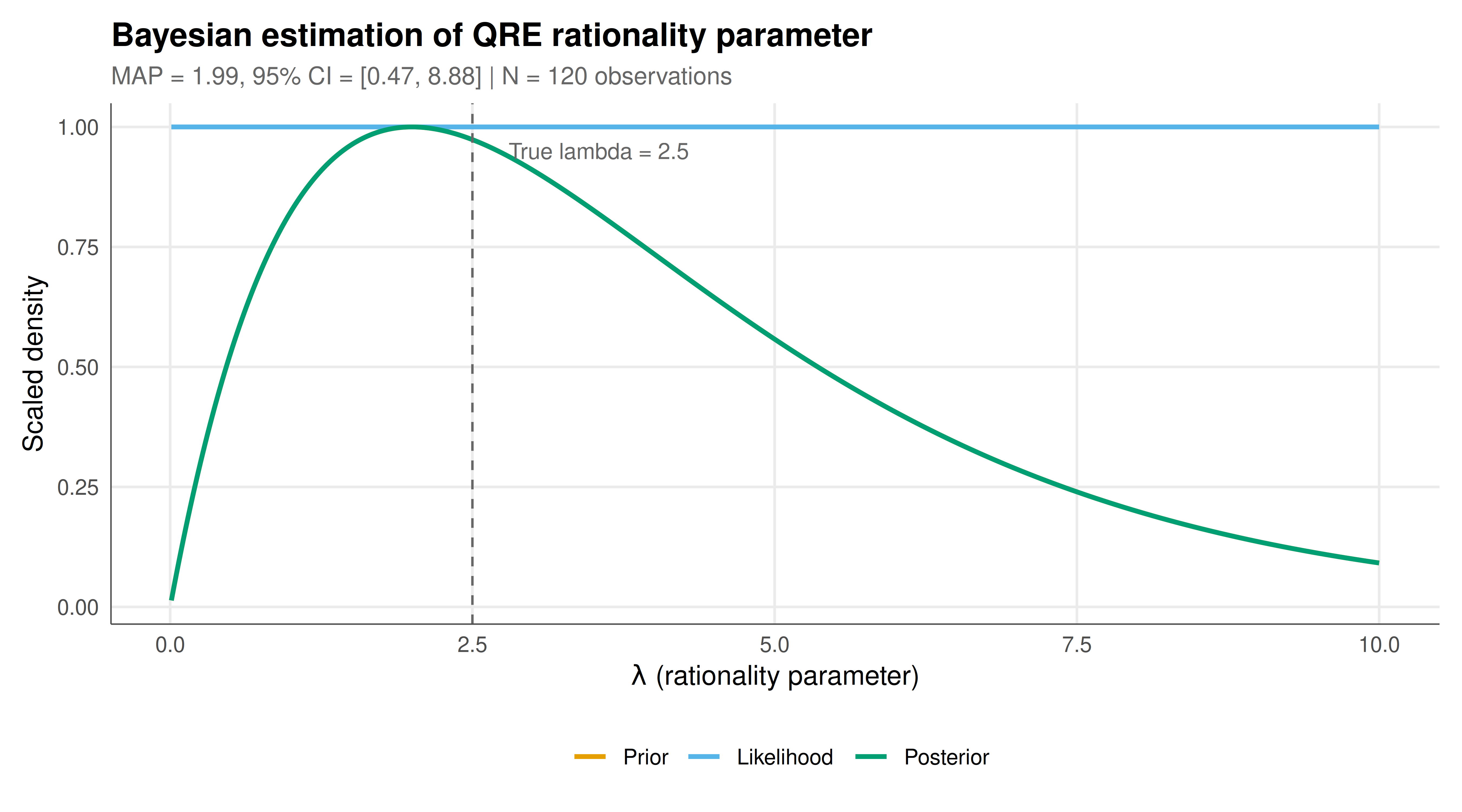
#| fig-cap: "Prior, likelihood, and posterior distributions for the QRE rationality parameter lambda. The prior (Gamma(2, 0.5)) is diffuse, the likelihood peaks near the data-generating value, and the posterior combines both sources of information. The vertical dashed line marks the true parameter value. Distributions are scaled to unit maximum for visual comparison. Rendered using the Okabe-Ito palette."
#| fig-width: 9
#| fig-height: 5
#| dev: [png, pdf]
#| dpi: 300
post_long <- posterior_df |>
  pivot_longer(cols = c(prior, likelihood, posterior),
               names_to = "distribution", values_to = "density") |>
  mutate(distribution = factor(distribution,
                               levels = c("prior", "likelihood", "posterior"),
                               labels = c("Prior", "Likelihood", "Posterior")))

ggplot(post_long, aes(x = lambda, y = density, color = distribution)) +
  geom_line(linewidth = 1) +
  geom_vline(xintercept = lambda_true, linetype = "dashed",
             color = "grey40", linewidth = 0.5) +
  annotate("text", x = lambda_true + 0.3, y = 0.95,
           label = paste0("True lambda = ", lambda_true),
           hjust = 0, size = 3.5, color = "grey40") +
  scale_color_manual(values = okabe_ito[c(1, 2, 3)], name = "") +
  labs(title = "Bayesian estimation of QRE rationality parameter",
       subtitle = sprintf("MAP = %.2f, 95%% CI = [%.2f, %.2f] | N = %d observations",
                          lambda_map, ci_low, ci_high, n_obs),
       x = expression(lambda ~ "(rationality parameter)"),
       y = "Scaled density") +
  theme_publication()
```
## Interactive figure
```{r}
#| label: fig-qre-probs-interactive
#| fig-cap: "Interactive plot showing how QRE choice probabilities change as a function of the rationality parameter lambda."
qre_curve <- data.frame(lambda = lambda_grid)
probs_mat <- t(sapply(lambda_grid, function(l) compute_qre(l, payoff_matrix)))
colnames(probs_mat) <- paste0("Strategy ", 1:3)
qre_curve <- cbind(qre_curve, as.data.frame(probs_mat))

qre_long <- qre_curve |>
  pivot_longer(cols = starts_with("Strategy"),
               names_to = "strategy", values_to = "probability")

p <- ggplot(qre_long, aes(x = lambda, y = probability, color = strategy,
                           text = paste0("Lambda: ", round(lambda, 2),
                                         "\n", strategy,
                                         "\nProbability: ",
                                         round(probability, 4)))) +
  geom_line(linewidth = 0.8) +
  geom_vline(xintercept = lambda_true, linetype = "dashed",
             color = "grey50", linewidth = 0.4) +
  scale_color_manual(values = okabe_ito[1:3], name = "Strategy") +
  labs(title = "QRE choice probabilities by rationality level",
       subtitle = "Hover to see exact probabilities at each lambda value",
       x = expression(lambda), y = "Choice probability") +
  theme_publication()

ggplotly(p, tooltip = "text") |>
  config(displaylogo = FALSE,
         modeBarButtonsToRemove = c("select2d", "lasso2d"))
```
## Interpretation
The Bayesian analysis successfully recovers the true rationality parameter from the simulated experimental data, demonstrating both the feasibility and the interpretive advantages of the Bayesian approach to game-theoretic estimation. The posterior distribution concentrates around the true value of $\lambda = 2.5$, with the MAP estimate and posterior mean both close to this value. The 95% credible interval provides a direct probability statement about where the true parameter lies, given the data and prior -- a more intuitive interpretation than the frequentist confidence interval, which describes the coverage property of a procedure across hypothetical replications.
The interplay between prior and likelihood is visible in the static figure. The Gamma(2, 0.5) prior is relatively diffuse, placing substantial probability mass across a wide range of $\lambda$ values. The likelihood, shaped by the 120 observed strategy choices, is more concentrated and dominates the posterior. This is the expected behavior when the sample size is moderately large relative to the prior's informativeness. In the small-sample regime common in laboratory experiments (say, 20-30 observations), the prior would exert more influence, and the choice of prior would matter more for the conclusions. The sensitivity of posteriors to prior choice in small samples is not a weakness of the Bayesian approach but rather an honest reflection of the limited information in the data -- information that frequentist methods can obscure through apparently precise point estimates.
The interactive figure reveals the rich structure of the QRE model by tracing choice probabilities as functions of $\lambda$. At $\lambda = 0$, all three strategies are played with equal probability (1/3), reflecting completely random behavior. As $\lambda$ increases, the probabilities begin to separate as more rational players increasingly favor higher-expected-payoff strategies. The specific shape of these probability curves depends on the payoff matrix: in our Rock-Paper-Scissors-like game with asymmetric payoffs, the symmetric QRE probabilities at low $\lambda$ give way to an asymmetric distribution as rationality increases. The transition reveals which strategies benefit most from increased strategic sophistication -- information that is valuable for predicting behavior across different subject populations or experimental conditions.
From a practical standpoint, the grid approximation method used here is suitable for low-dimensional problems (one or two parameters) and has the advantage of being completely transparent -- every step of the computation is visible and verifiable. For higher-dimensional problems involving multiple game parameters (e.g., separate rationality parameters for different player types, risk aversion coefficients, or altruism parameters), Markov chain Monte Carlo methods become necessary. The conceptual framework remains the same: specify a prior, define the likelihood through the game-theoretic model, and compute the posterior. The Bayesian approach also naturally handles model comparison through Bayes factors, enabling researchers to test whether the data better support a QRE model versus a Nash equilibrium model, or a model with homogeneous versus heterogeneous rationality levels. This model comparison capability makes Bayesian inference a comprehensive toolkit for empirical game theory, not merely a parameter estimation technique.
## Extensions & related tutorials
- [Cointegration analysis of strategic long-run relationships](../../time-series-econometrics/cointegration-strategic-long-run/) -- Apply time-series methods to estimate dynamic game parameters.
- [Cellular automata and spatial game theory](../../simulations/cellular-automata-game-theory/) -- Simulate games where Bayesian updating occurs in spatial populations.
- [Network visualization for games with igraph](../../visualization-and-communication/network-visualization-igraph/) -- Visualize posterior networks of game-theoretic parameters.
- [Uber surge pricing as a dynamic game](../../real-world-data-applications/uber-surge-pricing-game/) -- Estimate platform market parameters using observed pricing data.
- [Literate programming for game theory](../../reproducibility-open-science/literate-programming-game-theory/) -- Document Bayesian analyses reproducibly.
## References
::: {#refs}
:::