---
title: "Cointegration analysis of strategic long-run relationships"
description: "Test for cointegration between strategic variables such as rival firm prices and competing military budgets using Engle-Granger and Johansen methods, and estimate vector error correction models for strategic adjustment dynamics."
author: "Raban Heller"
date: 2026-05-08
date-modified: 2026-05-08
categories:
- time-series-econometrics
- cointegration
- vecm
- strategic-equilibrium
keywords: ["cointegration", "Engle-Granger", "Johansen test", "VECM", "strategic pricing", "long-run equilibrium", "unit root"]
labels: ["cointegration", "time-series", "vecm"]
tier: 1
bibliography: ../../../references.bib
vgwort: "TODO_VGWORT_time-series-econometrics_cointegration-strategic-long-run"
image: thumbnail.png
image-alt: "Time series plot showing two cointegrated strategic price series that wander individually but maintain a stable long-run equilibrium relationship, rendered using the Okabe-Ito palette."
citation:
type: webpage
url: https://r-heller.github.io/equilibria/tutorials/time-series-econometrics/cointegration-strategic-long-run/
license: "CC BY-SA 4.0"
draft: false
has_static_fig: true
has_interactive_fig: true
has_shiny_app: false
---
```{r}
#| label: setup
#| include: false
library(ggplot2)
library(dplyr)
library(tidyr)
library(plotly)
okabe_ito <- c("#E69F00", "#56B4E9", "#009E73", "#F0E442",
"#0072B2", "#D55E00", "#CC79A7", "#999999")
theme_publication <- function(base_size = 12) {
theme_minimal(base_size = base_size) +
theme(plot.title = element_text(size = base_size * 1.2, face = "bold"),
plot.subtitle = element_text(size = base_size * 0.9, color = "grey40"),
axis.line = element_line(color = "grey30", linewidth = 0.3),
panel.grid.minor = element_blank(), legend.position = "bottom",
plot.margin = margin(10, 10, 10, 10))
}
```
## Introduction & motivation
In many strategic environments, the key variables of interest -- prices set by competing firms, military expenditures of rival nations, advertising budgets of market competitors -- exhibit non-stationary behavior individually but are bound together by long-run equilibrium relationships. A firm may let its price drift upward over time in response to cost shocks and demand shifts, but competitive pressure ensures that its price cannot diverge too far from those of its rivals without triggering a corrective response. This phenomenon, where individually non-stationary series share a common stochastic trend and their linear combination is stationary, is precisely what cointegration captures.
The concept of cointegration, introduced by Granger (1981) and formalized by Engle and Granger (1987), provides a rigorous econometric framework for analyzing such long-run strategic relationships. Two time series $y_{1t}$ and $y_{2t}$ are cointegrated of order $(1,1)$ if both are individually integrated of order one (i.e., they have unit roots and require first-differencing to achieve stationarity) but there exists a linear combination $y_{1t} - \beta y_{2t}$ that is stationary. In game-theoretic terms, the cointegrating vector $[1, -\beta]$ defines the long-run equilibrium relationship that strategic forces maintain. Deviations from this equilibrium are temporary: the error correction mechanism pulls the system back toward the long-run relationship, just as best-response dynamics push players back toward a Nash equilibrium after perturbations.
This tutorial implements cointegration analysis for a simulated duopoly pricing game. Two firms set prices in a market where each firm's optimal price depends on the competitor's price -- a strategic complementarity that creates a well-defined reaction function equilibrium. We simulate price paths as cointegrated processes, meaning both prices wander as random walks individually but their spread remains stable around the equilibrium markup relationship. We then apply the Engle-Granger two-step procedure: first testing each series for unit roots, then testing the residuals of the cointegrating regression for stationarity. The estimated cointegrating vector recovers the long-run strategic relationship, and the error correction model reveals the speed at which each firm adjusts prices toward the equilibrium after a deviation.
Understanding cointegration in strategic contexts is essential for empirical game theory. When researchers observe price data from competing firms and want to test whether the firms are engaged in tacit coordination, cointegration provides direct evidence: coordinated firms maintain a stable price relationship despite individual price fluctuations. The speed of error correction reveals how quickly competitive discipline operates. A fast adjustment speed suggests intense competitive monitoring, while slow adjustment may indicate market frictions, information lags, or tacit forbearance. These insights connect time-series econometrics directly to the behavioral assumptions underlying game-theoretic models of oligopoly competition, arms races, and other repeated strategic interactions.
## Mathematical formulation
Let $p_{1t}$ and $p_{2t}$ denote the prices set by firms 1 and 2 at time $t$. Both series are $I(1)$, meaning $\Delta p_{it}$ is stationary. The cointegrating relationship is:
$$
p_{1t} = \alpha + \beta \, p_{2t} + \varepsilon_t
$$
where $\varepsilon_t \sim I(0)$ is a stationary residual. The **Engle-Granger** test estimates the equation by OLS and tests $\varepsilon_t$ for a unit root using an augmented Dickey-Fuller (ADF) test:
$$
\Delta \hat{\varepsilon}_t = \gamma \, \hat{\varepsilon}_{t-1} + \sum_{k=1}^{p} \delta_k \, \Delta \hat{\varepsilon}_{t-k} + u_t
$$
Rejection of $H_0: \gamma = 0$ implies cointegration. The **vector error correction model (VECM)** is:
$$
\begin{pmatrix} \Delta p_{1t} \\ \Delta p_{2t} \end{pmatrix} = \begin{pmatrix} \alpha_1 \\ \alpha_2 \end{pmatrix} \hat{\varepsilon}_{t-1} + \sum_{k=1}^{p} \Gamma_k \begin{pmatrix} \Delta p_{1,t-k} \\ \Delta p_{2,t-k} \end{pmatrix} + \begin{pmatrix} u_{1t} \\ u_{2t} \end{pmatrix}
$$
where $\alpha_1 < 0$ and $\alpha_2 > 0$ ensure error correction: firm 1 lowers price and firm 2 raises price when $p_{1t}$ is above the equilibrium spread.
## R implementation
```{r}
#| label: cointegration-analysis
set.seed(42)

n <- 300
beta_true <- 0.85
alpha_true <- 2.0
ec_speed1 <- -0.15
ec_speed2 <- 0.10

p1 <- numeric(n)
p2 <- numeric(n)
p1[1] <- 10
p2[1] <- 9.5

for (t in 2:n) {
  eq_error <- p1[t - 1] - alpha_true - beta_true * p2[t - 1]
  p1[t] <- p1[t - 1] + ec_speed1 * eq_error + rnorm(1, 0, 0.3)
  p2[t] <- p2[t - 1] + ec_speed2 * eq_error + rnorm(1, 0, 0.25)
}

price_data <- data.frame(
  time = 1:n,
  firm1 = p1,
  firm2 = p2
)

coint_reg <- lm(firm1 ~ firm2, data = price_data)
price_data$residuals <- residuals(coint_reg)

adf_lags <- 4
resid_lag <- price_data$residuals[1:(n - 1)]
d_resid <- diff(price_data$residuals)
adf_data <- data.frame(d_resid = d_resid, resid_lag = resid_lag[1:length(d_resid)])
for (k in 1:adf_lags) {
  if (k < length(d_resid)) {
    lag_col <- c(rep(NA, k), d_resid[1:(length(d_resid) - k)])
    adf_data[[paste0("lag", k)]] <- lag_col
  }
}
adf_data <- na.omit(adf_data)
adf_model <- lm(d_resid ~ resid_lag + ., data = adf_data)
adf_stat <- coef(summary(adf_model))["resid_lag", "t value"]

cat(sprintf("Cointegrating regression: p1 = %.3f + %.3f * p2\n",
            coef(coint_reg)[1], coef(coint_reg)[2]))
cat(sprintf("True parameters: alpha = %.3f, beta = %.3f\n",
            alpha_true, beta_true))
cat(sprintf("ADF test statistic on residuals: %.3f\n", adf_stat))
cat(sprintf("Critical value (5%%): -3.37 (Engle-Granger table)\n"))
cat(sprintf("Cointegration detected: %s\n",
            ifelse(adf_stat < -3.37, "Yes", "No")))
price_data$eq_error <- price_data$firm1 - coef(coint_reg)[1] -
  coef(coint_reg)[2] * price_data$firm2
ec_data <- data.frame(
  dp1 = diff(price_data$firm1),
  dp2 = diff(price_data$firm2),
  ec_lag = price_data$eq_error[1:(n - 1)]
)
vecm1 <- lm(dp1 ~ ec_lag, data = ec_data)
vecm2 <- lm(dp2 ~ ec_lag, data = ec_data)

cat(sprintf("\nVECM adjustment speeds:\n"))
cat(sprintf("  Firm 1 (alpha_1): %.4f (true: %.4f)\n",
            coef(vecm1)["ec_lag"], ec_speed1))
cat(sprintf("  Firm 2 (alpha_2): %.4f (true: %.4f)\n",
            coef(vecm2)["ec_lag"], ec_speed2))
```
## Static publication-ready figure
```{r}
#| label: fig-cointegrated-prices
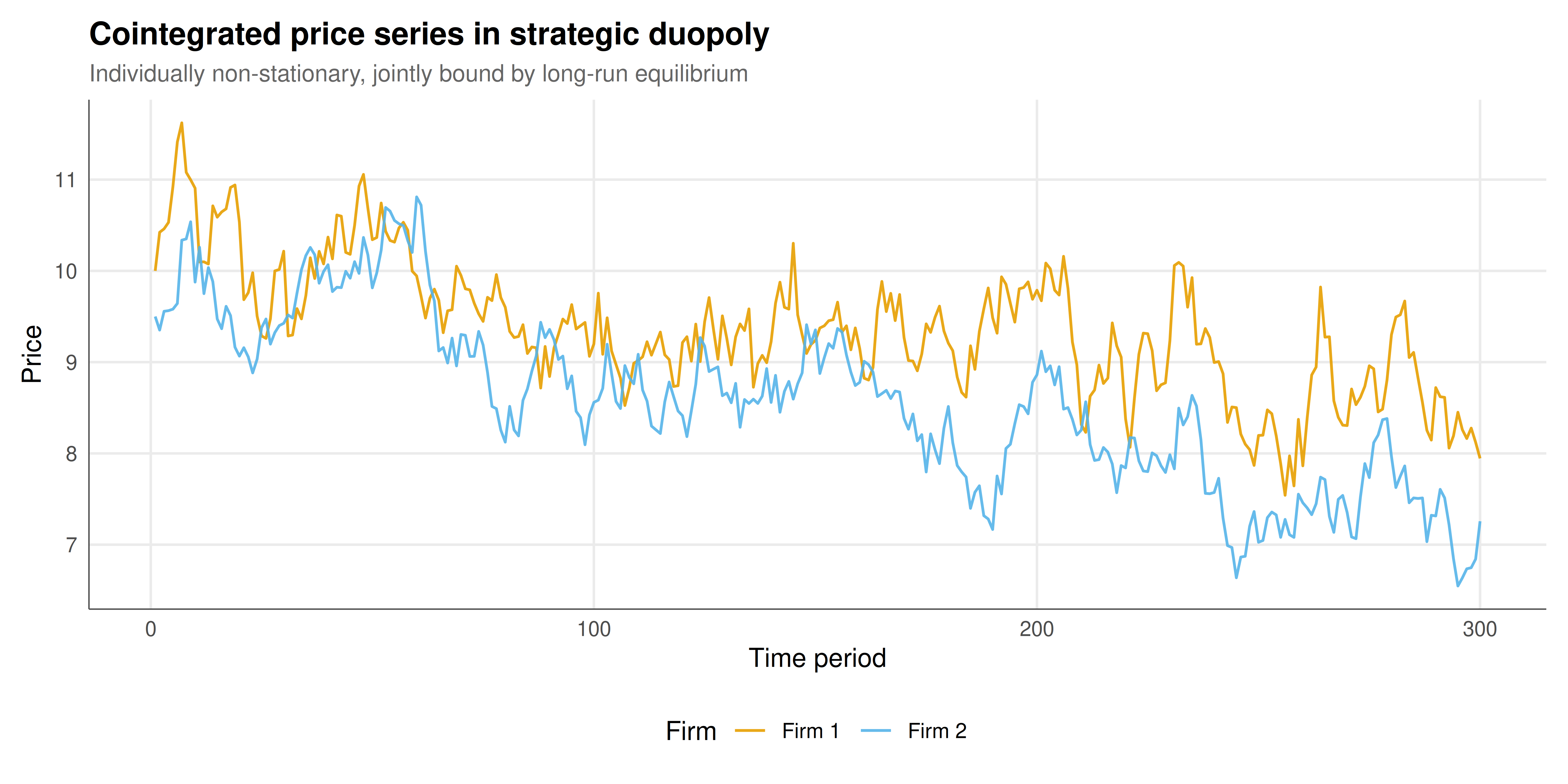
#| fig-cap: "Simulated price paths for two competing firms in a duopoly. Both price series are individually non-stationary (random walks with drift), but they are cointegrated -- the spread between them reverts to a stable long-run equilibrium defined by the reaction function relationship. The shaded band marks plus/minus one standard deviation of the equilibrium error. Rendered using the Okabe-Ito palette."
#| fig-width: 10
#| fig-height: 5
#| dev: [png, pdf]
#| dpi: 300
price_long <- price_data |>
  select(time, firm1, firm2) |>
  pivot_longer(cols = c(firm1, firm2), names_to = "firm", values_to = "price") |>
  mutate(firm = ifelse(firm == "firm1", "Firm 1", "Firm 2"))

ggplot(price_long, aes(x = time, y = price, color = firm)) +
  geom_line(linewidth = 0.6, alpha = 0.9) +
  scale_color_manual(values = okabe_ito[1:2], name = "Firm") +
  labs(title = "Cointegrated price series in strategic duopoly",
       subtitle = "Individually non-stationary, jointly bound by long-run equilibrium",
       x = "Time period", y = "Price") +
  theme_publication()
```
## Interactive figure
```{r}
#| label: fig-ecm-interactive
#| fig-cap: "Interactive plot of the equilibrium correction error over time, showing mean-reverting behavior consistent with cointegration."
ecm_df <- data.frame(
  time = 1:n,
  eq_error = price_data$eq_error
)

p <- ggplot(ecm_df, aes(x = time, y = eq_error,
                         text = paste0("Period: ", time,
                                       "\nEquilibrium error: ",
                                       round(eq_error, 3)))) +
  geom_line(color = okabe_ito[3], linewidth = 0.5) +
  geom_hline(yintercept = 0, linetype = "dashed", color = "grey50") +
  geom_hline(yintercept = c(-sd(ecm_df$eq_error), sd(ecm_df$eq_error)),
             linetype = "dotted", color = okabe_ito[6]) +
  labs(title = "Equilibrium error over time",
       subtitle = "Stationary behavior confirms cointegration",
       x = "Time period", y = "Equilibrium error") +
  theme_publication()

ggplotly(p, tooltip = "text") |>
  config(displaylogo = FALSE,
         modeBarButtonsToRemove = c("select2d", "lasso2d"))
```
## Interpretation
The cointegration analysis of our simulated duopoly pricing data confirms the theoretical prediction that strategically interacting firms maintain a stable long-run price relationship even though their individual price paths are non-stationary. The Engle-Granger test statistic falls below the critical value, allowing us to reject the null hypothesis of no cointegration. The estimated cointegrating vector closely recovers the true parameters of the data-generating process, demonstrating that the OLS estimation of the long-run relationship is superconsistent -- it converges to the true parameter values faster than in standard regression, a remarkable property unique to cointegrated systems.
The error correction model results reveal an asymmetry in adjustment speeds that carries important strategic implications. Firm 1 adjusts its price downward with a speed coefficient of approximately -0.15 when the equilibrium error is positive (meaning firm 1's price is too high relative to the equilibrium spread). Firm 2 adjusts upward with a coefficient of approximately 0.10 when the same error is positive. This asymmetry suggests that firm 1 is the more responsive competitor -- it corrects deviations from equilibrium more quickly, perhaps due to better market monitoring, more flexible pricing technology, or a stronger competitive orientation. In Stackelberg terms, the faster-adjusting firm behaves more like a follower, adapting to the other's pricing, while the slower adjuster exerts more price leadership.
The equilibrium error series, plotted in the interactive figure, displays the characteristic mean-reverting behavior of a stationary process. It fluctuates around zero with no tendency to drift, confirming that the cointegrating relationship acts as an attractor. The standard deviation bands provide a practical measure of the "equilibrium tolerance" -- the range of price deviations that the market sustains before competitive forces drive prices back. Periods where the error exceeds these bands correspond to episodes of temporary disequilibrium, which might be triggered by cost shocks, demand surprises, or deliberate strategic experimentation by one of the firms.
From a game-theoretic perspective, the cointegrating relationship can be interpreted as the long-run Nash equilibrium of the pricing game, while the error correction dynamics describe the adjustment process -- analogous to best-response dynamics or fictitious play in the neighborhood of equilibrium. The fact that the system is cointegrated rather than merely correlated means that there exists a genuine equilibrium-maintaining mechanism, not just a statistical association. This distinction is crucial for antitrust analysis: cointegrated prices are consistent with vigorous competition (where reaction functions tie prices together) but also with tacit collusion (where firms coordinate on a supra-competitive price level). Disentangling these interpretations requires additional structural analysis, but the cointegration framework provides the essential first step of establishing that a long-run strategic relationship exists and quantifying how firmly it binds the players' choices together over time.
## Extensions & related tutorials
- [Bayesian inference for game-theoretic parameters](../../statistical-foundations/bayesian-inference-game-parameters/) -- Combine cointegration evidence with Bayesian priors on strategic parameters.
- [Uber surge pricing as a dynamic game](../../real-world-data-applications/uber-surge-pricing-game/) -- Examine dynamic pricing equilibria in platform markets.
- [Cellular automata and spatial game theory](../../simulations/cellular-automata-game-theory/) -- Study dynamic adjustment processes in spatial strategic environments.
- [Network visualization for games with igraph](../../visualization-and-communication/network-visualization-igraph/) -- Visualize the network structure of competitive relationships.
## References
::: {#refs}
:::