---
title: "Global games and coordination under private information"
description: "Implement the Carlsson-van Damme and Morris-Shin global games framework in R, showing how private noisy signals about fundamentals resolve equilibrium multiplicity in coordination games through threshold strategies."
author: "Raban Heller"
date: 2026-05-08
date-modified: 2026-05-08
categories:
- bayesian-methods
- global-games
- coordination
- incomplete-information
keywords: ["global games", "coordination game", "private information", "threshold strategy", "Morris-Shin", "currency attack", "equilibrium uniqueness"]
labels: ["bayesian-games", "equilibrium-selection"]
tier: 1
bibliography: ../../../references.bib
vgwort: "TODO_VGWORT_bayesian-methods_global-games-coordination"
image: thumbnail.png
image-alt: "Threshold strategy diagram showing attack probability as a function of private signal in a global game"
citation:
type: webpage
url: https://r-heller.github.io/equilibria/tutorials/bayesian-methods/global-games-coordination/
license: "CC BY-SA 4.0"
draft: false
has_static_fig: true
has_interactive_fig: true
has_shiny_app: false
---
```{r}
#| label: setup
#| include: false
library(ggplot2)
library(dplyr)
library(tidyr)
library(plotly)
okabe_ito <- c("#E69F00", "#56B4E9", "#009E73", "#F0E442",
"#0072B2", "#D55E00", "#CC79A7", "#999999")
theme_publication <- function(base_size = 12) {
theme_minimal(base_size = base_size) +
theme(
plot.title = element_text(size = base_size * 1.2, face = "bold"),
plot.subtitle = element_text(size = base_size * 0.9, color = "grey40"),
axis.line = element_line(color = "grey30", linewidth = 0.3),
panel.grid.minor = element_blank(),
legend.position = "bottom",
plot.margin = margin(10, 10, 10, 10)
)
}
```
## Introduction & motivation
Coordination games with multiple equilibria pose a fundamental challenge for economic theory: if a game has two or more Nash equilibria, which one will players select? The standard model of a bank run, a currency crisis, or a debt rollover problem features two equilibria -- a good one (no attack, no run) and a bad one (attack, run) -- and the theory is silent on when each occurs. This multiplicity problem plagued macroeconomic models of financial crises throughout the 1980s and 1990s, limiting their predictive and policy-relevant content. If a currency crisis can happen in any equilibrium, the model cannot tell us which fundamentals make crises more likely.
The **global games** framework, pioneered by Carlsson and van Damme (1993) and applied to macroeconomic settings by Morris and Shin (1998, 2003), provides an elegant resolution. The key innovation is to introduce a small amount of **private information**: instead of fundamentals being common knowledge, each player observes a noisy private signal about the true state of the economy. This seemingly minor perturbation has dramatic consequences -- the game that had multiple equilibria under common knowledge now has a **unique equilibrium** in threshold strategies. Each player attacks (withdraws, speculates against the currency) if and only if their private signal falls below a critical threshold, and this threshold is uniquely determined by the model parameters.
The intuition for uniqueness is subtle and powerful. Under common knowledge, players can coordinate on either equilibrium because they all share the same information. With private signals, each player is uncertain about what others observe, which destroys the ability to coordinate on the "good" equilibrium in states where fundamentals are weak. The resulting threshold equilibrium has a natural interpretation: the attack succeeds (the bank fails, the currency devalues) when the fundamental is below a critical value that depends on the noise precision. As signals become more precise, the threshold converges to the point where fundamentals alone determine the outcome, independent of expectations. As signals become noisier, the threshold shifts toward the risk-dominant equilibrium of the underlying complete-information game. This tutorial implements the Morris-Shin currency attack model, derives the equilibrium threshold analytically, and visualises how signal precision shapes the boundary between crisis and stability. The global games approach has become one of the most widely used tools in modern financial economics, applied to bank runs, sovereign debt crises, corporate finance, and political regime change.
## Mathematical formulation
Consider a continuum of agents indexed on $[0, 1]$. The true fundamental is $\theta \sim \text{Uniform}[\underline{\theta}, \overline{\theta}]$. Each agent $i$ observes a private signal:
$$
x_i = \theta + \varepsilon_i, \quad \varepsilon_i \sim N(0, \sigma^2)
$$
where $\varepsilon_i$ are i.i.d. and independent of $\theta$. Each agent chooses to **attack** ($a_i = 1$) or **not attack** ($a_i = 0$). Let $\ell = \int_0^1 a_i \, di$ be the fraction of agents who attack.
The attack **succeeds** (regime change, currency devaluation, bank failure) if and only if $\ell \geq \theta$ -- the proportion of attackers exceeds the fundamental strength. Payoffs:
$$
u_i(a_i, \ell, \theta) = \begin{cases}
1 - c & \text{if } a_i = 1 \text{ and attack succeeds } (\ell \geq \theta) \\
-c & \text{if } a_i = 1 \text{ and attack fails } (\ell < \theta) \\
0 & \text{if } a_i = 0
\end{cases}
$$
where $c \in (0, 1)$ is the cost of attacking.
**Threshold equilibrium**: In the unique equilibrium, agent $i$ attacks if and only if $x_i < x^*$, where $x^*$ is the equilibrium signal threshold. The **equilibrium threshold** and the **critical fundamental** $\theta^*$ (below which the regime falls) satisfy:
$$
\theta^* = 1 - \Phi\!\left(\frac{\theta^* - x^*}{\sigma}\right), \quad
\Phi\!\left(\frac{x^* - \theta^*}{\sigma}\right) = 1 - c
$$
where $\Phi$ is the standard normal CDF. Combining these conditions:
$$
x^* = \theta^* + \sigma \, \Phi^{-1}(1 - c)
$$
and $\theta^*$ solves:
$$
\theta^* = 1 - \Phi\!\left(-\Phi^{-1}(1 - c)\right) = c
$$
In the limit of precise signals ($\sigma \to 0$), the fundamental threshold is $\theta^* = c$: the regime falls if and only if the fundamental is below the attack cost. This is the **unique equilibrium** of the global game.
## R implementation
```{r}
#| label: global-games-analysis
# Morris-Shin global game: currency attack model
global_game_threshold <- function(c_cost, sigma) {
  # Equilibrium fundamental threshold
  theta_star <- c_cost

  # Equilibrium signal threshold
  x_star <- theta_star + sigma * qnorm(1 - c_cost)

  # Probability of successful attack given theta
  prob_attack_succeeds <- function(theta) {
    # Fraction attacking = Prob(x_i < x_star | theta) = Phi((x_star - theta)/sigma)
    ell <- pnorm((x_star - theta) / sigma)
    # Attack succeeds if ell >= theta
    as.numeric(ell >= theta)
  }

  list(theta_star = theta_star, x_star = x_star, c_cost = c_cost, sigma = sigma)
}

cat("=== Global Game: Currency Attack Model ===\n")
for (sigma in c(0.1, 0.5, 1.0, 2.0)) {
  result <- global_game_threshold(c_cost = 0.3, sigma = sigma)
  cat(sprintf("sigma = %.1f: theta* = %.3f, x* = %.3f\n",
              sigma, result$theta_star, result$x_star))
}
cat("\n=== How attack cost affects equilibrium ===\n")
for (c_cost in c(0.1, 0.3, 0.5, 0.7, 0.9)) {
  result <- global_game_threshold(c_cost = c_cost, sigma = 0.5)
  cat(sprintf("c = %.1f: theta* = %.3f, x* = %.3f\n",
              c_cost, result$theta_star, result$x_star))
}
# Simulate the global game
cat("\n=== Simulation: N = 1000 agents, sigma = 0.3 ===\n")
set.seed(42)
N_agents <- 1000
sigma <- 0.3
c_cost <- 0.3

result <- global_game_threshold(c_cost, sigma)

# Simulate for different true fundamentals
for (theta_true in c(0.1, 0.3, 0.5, 0.7)) {
  signals <- theta_true + rnorm(N_agents, 0, sigma)
  attacks <- signals < result$x_star
  frac_attacking <- mean(attacks)
  regime_falls <- frac_attacking >= theta_true

  cat(sprintf("theta = %.1f: %.1f%% attack, regime %s (threshold: %.1f%%)\n",
              theta_true, 100 * frac_attacking,
              ifelse(regime_falls, "FALLS", "survives"),
              100 * theta_true))
}
# Expected payoff from attacking given signal x
cat("\n=== Expected payoff from attacking given signal ===\n")
expected_payoff_attack <- function(x, c_cost, sigma) {
  # E[u | attack, x] = Prob(regime falls | x) * (1-c) + Prob(survives | x) * (-c)
  # Prob(regime falls | x) = Prob(theta < theta* | x) by the equilibrium characterization
  # In the limit, this simplifies. For the exact calculation:
  # Agent believes theta | x ~ N(x, sigma^2) (with uniform prior approximation)
  # Regime falls when theta < theta_star = c
  prob_falls <- pnorm((c_cost - x) / sigma)
  prob_falls * (1 - c_cost) + (1 - prob_falls) * (-c_cost)
}

x_vals <- c(0.0, 0.15, 0.30, 0.45, 0.60)
for (x in x_vals) {
  ep <- expected_payoff_attack(x, c_cost, sigma)
  cat(sprintf("  x = %.2f: E[payoff|attack] = %+.4f -> %s\n",
              x, ep, ifelse(ep > 0, "ATTACK", "don't attack")))
}
```
## Static publication-ready figure
```{r}
#| label: fig-global-games-threshold
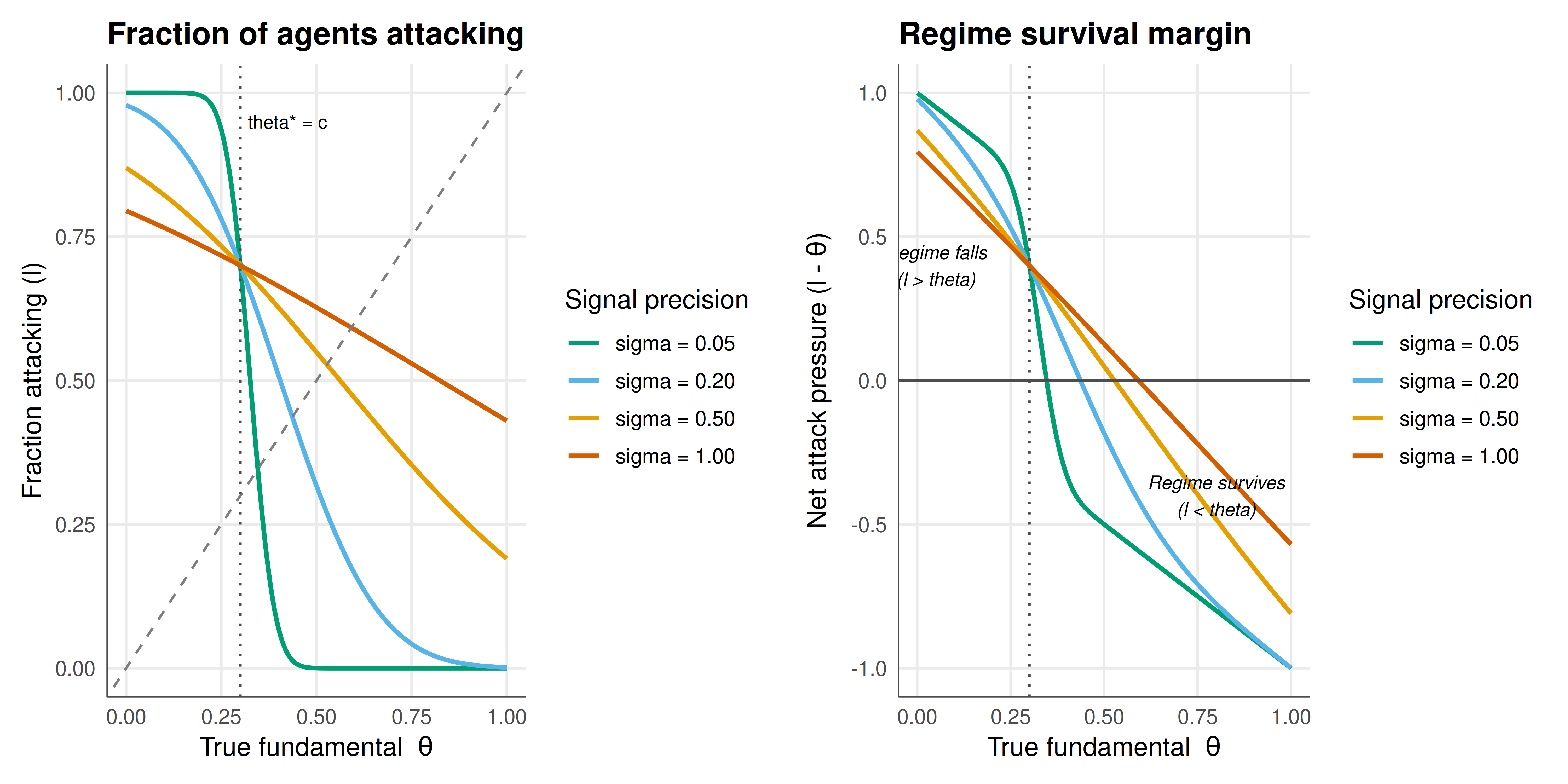
#| fig-cap: "Figure 1. Global game equilibrium: attack probability and regime survival as a function of the true fundamental theta, for varying signal precision. Left panel: fraction of agents who attack in equilibrium (agents with signals below x* attack). Right panel: regime outcome (falls if attack fraction exceeds theta). As precision increases (sigma decreases), the transition sharpens around theta* = c = 0.3, approaching a knife-edge where fundamentals alone determine the outcome. Okabe-Ito palette."
#| dev: [png, pdf]
#| fig-width: 10
#| fig-height: 5
#| dpi: 300
c_cost <- 0.3
theta_grid <- seq(-0.5, 1.5, by = 0.005)
sigma_vals <- c(0.05, 0.2, 0.5, 1.0)

attack_data <- bind_rows(lapply(sigma_vals, function(s) {
  res <- global_game_threshold(c_cost, s)
  # Fraction attacking = Phi((x* - theta) / sigma)
  frac_attack <- pnorm((res$x_star - theta_grid) / s)
  tibble(
    theta = theta_grid,
    frac_attack = frac_attack,
    regime_falls = as.numeric(frac_attack >= theta_grid),
    sigma_label = sprintf("sigma = %.2f", s),
    sigma = s
  )
}))

attack_data$sigma_label <- factor(attack_data$sigma_label,
                                    levels = sprintf("sigma = %.2f", sigma_vals))

# Left panel: fraction attacking
p_left <- ggplot(attack_data |> filter(theta >= 0, theta <= 1),
                  aes(x = theta, y = frac_attack, color = sigma_label)) +
  geom_line(linewidth = 1) +
  geom_abline(slope = 1, intercept = 0, linetype = "dashed", color = "grey50") +
  geom_vline(xintercept = c_cost, linetype = "dotted", color = "grey30") +
  annotate("text", x = c_cost + 0.02, y = 0.95, label = "theta* = c",
           size = 3, hjust = 0) +
  scale_color_manual(values = okabe_ito[c(3, 2, 1, 6)], name = "Signal precision") +
  labs(
    title = "Fraction of agents attacking",
    x = expression(paste("True fundamental  ", theta)),
    y = "Fraction attacking (l)"
  ) +
  theme_publication() +
  theme(legend.position = "right")

# Right panel: regime outcome boundary
boundary_data <- attack_data |>
  filter(theta >= 0, theta <= 1) |>
  mutate(net_attack = frac_attack - theta)  # positive = regime falls

p_right <- ggplot(boundary_data, aes(x = theta, y = net_attack, color = sigma_label)) +
  geom_line(linewidth = 1) +
  geom_hline(yintercept = 0, linetype = "solid", color = "grey30", linewidth = 0.5) +
  geom_vline(xintercept = c_cost, linetype = "dotted", color = "grey30") +
  annotate("text", x = 0.05, y = 0.4, label = "Regime falls\n(l > theta)",
           size = 3, fontface = "italic") +
  annotate("text", x = 0.8, y = -0.4, label = "Regime survives\n(l < theta)",
           size = 3, fontface = "italic") +
  scale_color_manual(values = okabe_ito[c(3, 2, 1, 6)], name = "Signal precision") +
  labs(
    title = "Regime survival margin",
    x = expression(paste("True fundamental  ", theta)),
    y = expression(paste("Net attack pressure (l - ", theta, ")"))
  ) +
  theme_publication() +
  theme(legend.position = "right")

# Combine using patchwork-free approach: side by side via grid
gridExtra::grid.arrange(p_left, p_right, ncol = 2)
```
## Interactive figure
```{r}
#| label: fig-global-games-interactive
# Interactive: signal threshold x* as function of sigma and c
param_data <- expand.grid(
  sigma = seq(0.01, 2, by = 0.05),
  c_cost = seq(0.1, 0.9, by = 0.1)
) |>
  mutate(
    theta_star = c_cost,
    x_star = theta_star + sigma * qnorm(1 - c_cost),
    text = paste0("sigma = ", round(sigma, 2),
                  "\nc = ", c_cost,
                  "\ntheta* = ", round(theta_star, 3),
                  "\nx* = ", round(x_star, 3))
  )

p_interactive <- ggplot(param_data, aes(x = sigma, y = x_star,
                                         color = factor(c_cost), text = text)) +
  geom_line(linewidth = 1) +
  geom_hline(yintercept = 0, linetype = "dashed", color = "grey50") +
  scale_color_manual(
    values = rep(okabe_ito, length.out = length(unique(param_data$c_cost))),
    name = "Attack cost (c)"
  ) +
  labs(
    title = "Signal threshold x* across parameter space",
    subtitle = "Higher noise (sigma) shifts threshold; higher cost reduces attacks",
    x = expression(paste("Signal noise (", sigma, ")")),
    y = "Signal threshold (x*)"
  ) +
  theme_publication()

ggplotly(p_interactive, tooltip = "text") |>
  config(displaylogo = FALSE,
         modeBarButtonsToRemove = c("select2d", "lasso2d"))
```
## Interpretation
The global games framework achieves something remarkable: it provides a principled, parameter-dependent answer to the question "when do coordination failures occur?" that the standard multiple-equilibria models cannot. The equilibrium threshold $\theta^* = c$ has a clean economic interpretation: the regime falls when the fundamental is below the attack cost. This means that in equilibrium, agents attack when -- and only when -- their private information suggests the fundamental is weak enough that the attack is likely to succeed. The self-fulfilling nature of crises is not eliminated but is disciplined: crises occur in a deterministic region of the fundamental space (for precise enough signals), and the width of the "crisis zone" depends on model parameters.
The visualisation of how signal precision affects the transition is particularly instructive. With very precise signals ($\sigma \to 0$), the fraction-attacking curve approaches a step function at $\theta^* = c$: below this threshold, essentially all agents attack; above it, essentially none do. Fundamentals alone determine the outcome. With imprecise signals ($\sigma$ large), the transition is gradual: even with moderately strong fundamentals, a non-trivial fraction of agents attack because their signals are noisy enough to suggest weakness. This gradualism means that the regime can fail at fundamentals above $\theta^*$ due to noise-induced coordination on the bad outcome.
The policy implications are profound. First, **transparency matters**: improving the quality of public information (reducing $\sigma$) sharpens the crisis boundary, making crises less likely for sound fundamentals but no less certain for unsound ones. Second, **the cost of attacking matters**: policies that raise the cost of speculation (capital controls, transaction taxes) shift $\theta^*$ downward, reducing the fundamental range over which crises occur. Third, unlike multiple-equilibria models where "animal spirits" or "sunspots" drive crises, the global games model makes crises **predictable** -- they are more likely when fundamentals are weak, noise is high, and attack costs are low. This predictability is what makes the framework valuable for empirical work and stress testing.
The connection to the underlying coordination game is also illuminating. Without private information, the game has two equilibria for intermediate fundamentals. The global game selects between them using a refinement that is robust to the details of the information structure -- the unique equilibrium converges to the risk-dominant equilibrium of the complete-information game as signals become noisy. This provides a game-theoretic foundation for risk dominance as a selection criterion.
## Extensions & related tutorials
- [Bank runs as a coordination game](../../classical-games/bank-runs-coordination/) -- the complete-information coordination game that global games refine.
- [Bayesian games and incomplete information](../bayesian-games-incomplete-information/) -- the general framework of games with private types.
- [The Stag Hunt — coordination, trust, and risk dominance](../../classical-games/stag-hunt/) -- the underlying coordination structure.
- [Signaling games and perfect Bayesian equilibrium](../../foundations/signaling-games-pbe/) -- another approach to games with private information.
- [Nash equilibrium in mixed strategies](../../foundations/nash-equilibrium-mixed/) -- mixed equilibria in the complete-information benchmark.
## References
::: {#refs}
:::