---
title: "Level-k thinking and cognitive hierarchy — bounded rationality in strategic games"
description: "Implement the level-k model and Camerer-Ho-Chong cognitive hierarchy for the p-beauty contest, simulate heterogeneous populations, and visualize convergence to Nash equilibrium as strategic sophistication increases."
author: "Raban Heller"
date: 2026-05-08
date-modified: 2026-05-08
categories:
- behavioral-gt
- level-k
- cognitive-hierarchy
- bounded-rationality
keywords: ["level-k model", "cognitive hierarchy", "p-beauty contest", "bounded rationality", "Camerer", "iterated reasoning"]
labels: ["behavioral-gt", "experimental-economics"]
tier: 1
bibliography: ../../../references.bib
vgwort: "TODO_VGWORT_behavioral-gt_level-k-cognitive-hierarchy"
image: thumbnail.png
image-alt: "Distribution of guesses in a p-beauty contest under the cognitive hierarchy model with different tau parameters"
citation:
type: webpage
url: https://r-heller.github.io/equilibria/tutorials/behavioral-gt/level-k-cognitive-hierarchy/
license: "CC BY-SA 4.0"
draft: false
has_static_fig: true
has_interactive_fig: true
has_shiny_app: false
---
```{r}
#| label: setup
#| include: false
library(ggplot2)
library(dplyr)
library(tidyr)
library(plotly)
okabe_ito <- c("#E69F00", "#56B4E9", "#009E73", "#F0E442",
"#0072B2", "#D55E00", "#CC79A7", "#999999")
theme_publication <- function(base_size = 12) {
theme_minimal(base_size = base_size) +
theme(plot.title = element_text(size = base_size * 1.2, face = "bold"),
plot.subtitle = element_text(size = base_size * 0.9, color = "grey40"),
axis.line = element_line(color = "grey30", linewidth = 0.3),
panel.grid.minor = element_blank(), legend.position = "bottom",
plot.margin = margin(10, 10, 10, 10))
}
```
## Introduction & motivation
Nash equilibrium assumes that all players are perfectly rational, that they correctly anticipate other players' strategies, and that these beliefs are mutually consistent. In practice, people engage in **limited depths of strategic reasoning**. In laboratory experiments, subjects rarely iterate beyond a few levels of reasoning, even in games where the Nash equilibrium requires infinite iterative elimination of dominated strategies. The **p-beauty contest** (or "guess 2/3 of the average" game) starkly illustrates this: Nash equilibrium predicts that everyone guesses 0, but experimental data consistently shows a wide distribution of guesses centred around 20--35, suggesting that most players perform only 1--3 steps of strategic reasoning.
The **level-k model**, formalised by @nagel_1995 and developed further by @stahl_wilson_1994 and @costa_gomes_crawford_2006, provides a structured framework for bounded rationality. It posits a hierarchy of player types: **Level-0 (L0)** players are non-strategic, typically modelled as randomising uniformly over available actions; **Level-1 (L1)** players best-respond to L0; **Level-2 (L2)** players best-respond to L1; and so on. Each level $k$ player assumes everyone else is exactly one level below them --- a strong but tractable assumption. In the beauty contest with $p = 2/3$, L0 guesses 50 (the midpoint), L1 guesses $50 \times 2/3 \approx 33.3$, L2 guesses $33.3 \times 2/3 \approx 22.2$, and the sequence converges geometrically to the Nash equilibrium of 0.
@camerer_ho_chong_2004 extended this with the **cognitive hierarchy (CH) model**, which relaxes the level-k assumption that each player believes everyone else is exactly one level below. Instead, a level-$k$ player in the CH model correctly anticipates the distribution of players at levels $0, 1, \ldots, k-1$ and best-responds to this mixture. The distribution of levels follows a Poisson distribution with parameter $\tau$, which captures the average depth of reasoning in the population. When $\tau$ is small, most players are L0 or L1; as $\tau \to \infty$, the distribution shifts toward higher levels and the aggregate prediction converges to Nash equilibrium. Empirically, $\tau \approx 1.5$ fits a wide range of experimental data across different games.
This tutorial implements both models for the p-beauty contest, simulates populations with heterogeneous reasoning depths, demonstrates how the aggregate guess distribution depends on $\tau$, and shows the convergence to Nash equilibrium. The analysis highlights a deep insight: the gap between Nash predictions and observed behaviour is not random noise but reflects the structured distribution of strategic sophistication in the population.
## Mathematical formulation
**Beauty contest.** $n$ players simultaneously choose a number $g_i \in [0, 100]$. The winner is the player whose guess is closest to $p \cdot \bar{g}$, where $\bar{g} = \frac{1}{n}\sum_i g_i$ and $p \in (0, 1)$. The unique Nash equilibrium is $g_i = 0$ for all $i$.
**Level-k model.** Define the hierarchy of best responses:
$$
g_0 = 50, \quad g_k = p \cdot g_{k-1} = 50 \cdot p^k \quad \text{for } k \geq 1
$$
In general, $g_k = 50 \cdot p^k \xrightarrow{k \to \infty} 0$, converging to the Nash equilibrium.
**Cognitive hierarchy model.** The fraction of players at level $k$ follows a Poisson distribution:
$$
f(k \mid \tau) = \frac{e^{-\tau} \tau^k}{k!}
$$
A level-$k$ player believes the population consists only of levels $0, 1, \ldots, k-1$, with normalised probabilities:
$$
g_k^{CH} = p \cdot \frac{\sum_{j=0}^{k-1} f(j \mid \tau) \cdot g_j^{CH}}{\sum_{j=0}^{k-1} f(j \mid \tau)}
$$
The aggregate predicted guess is:
$$
\bar{g}^{CH}(\tau) = \sum_{k=0}^{\infty} f(k \mid \tau) \cdot g_k^{CH}
$$
## R implementation
```{r}
#| label: level-k-and-ch
# --- Parameters ---
p <- 2/3         # beauty contest multiplier
g0 <- 50         # L0 guess (midpoint)
K_max <- 15      # maximum level to compute

# --- Level-k model ---
level_k_guesses <- function(p, g0, K) {
  guesses <- numeric(K + 1)
  guesses[1] <- g0  # L0

  for (k in 2:(K + 1)) {
    guesses[k] <- p * guesses[k - 1]
  }
  names(guesses) <- paste0("L", 0:K)
  guesses
}

lk_guesses <- level_k_guesses(p, g0, K_max)
cat("=== Level-k Guesses (p = 2/3) ===\n")
for (k in 0:8) {
  cat(sprintf("  L%d: %.4f\n", k, lk_guesses[k + 1]))
}
# --- Cognitive hierarchy model ---
ch_guesses <- function(p, g0, tau, K_max = 20) {
  # Poisson probabilities
  probs <- dpois(0:K_max, lambda = tau)

  # CH guesses: L0 is g0, Lk best-responds to the perceived mixture of 0..k-1
  g_ch <- numeric(K_max + 1)
  g_ch[1] <- g0

  for (k in 1:K_max) {
    # Weights for levels 0 to k-1 (normalised)
    w <- probs[1:k]
    w <- w / sum(w)
    # Expected average guess perceived by level k
    perceived_avg <- sum(w * g_ch[1:k])
    g_ch[k + 1] <- p * perceived_avg
  }

  names(g_ch) <- paste0("L", 0:K_max)
  list(guesses = g_ch, probs = probs)
}

cat("\n=== Cognitive Hierarchy Guesses (tau = 1.5) ===\n")
ch_15 <- ch_guesses(p, g0, tau = 1.5, K_max = K_max)
for (k in 0:8) {
  cat(sprintf("  L%d: guess=%.4f, prob=%.4f\n", k, ch_15$guesses[k + 1],
              ch_15$probs[k + 1]))
}
# Aggregate prediction
aggregate_guess <- function(tau, p = 2/3, g0 = 50, K_max = 20) {
  ch <- ch_guesses(p, g0, tau, K_max)
  sum(ch$probs * ch$guesses)
}

cat("\n=== Aggregate CH Prediction vs tau ===\n")
for (tau in c(0.5, 1.0, 1.5, 2.0, 3.0, 5.0, 10.0, 50.0)) {
  agg <- aggregate_guess(tau)
  cat(sprintf("  tau=%5.1f: aggregate guess = %.4f\n", tau, agg))
}
# --- Population simulation ---
set.seed(42)
simulate_ch_population <- function(n_players, tau, p = 2/3, g0 = 50, K_max = 20) {
  ch <- ch_guesses(p, g0, tau, K_max)
  # Assign levels to players
  levels <- rpois(n_players, lambda = tau)
  levels <- pmin(levels, K_max)
  # Get each player's guess
  guesses <- ch$guesses[levels + 1]
  # Add small noise for realism
  guesses <- pmax(0, pmin(100, guesses + rnorm(n_players, 0, 2)))
  data.frame(player = 1:n_players, level = levels, guess = guesses)
}

cat("\n=== Simulated Population (n=1000, tau=1.5) ===\n")
sim_data <- simulate_ch_population(1000, tau = 1.5)
cat(sprintf("  Mean guess: %.2f\n", mean(sim_data$guess)))
cat(sprintf(" Median guess: %.2f\n", median(sim_data$guess)))
cat(sprintf(" Target (2/3 * mean): %.2f\n", p * mean(sim_data$guess)))
cat(" Level distribution:\n")
level_tab <- table(sim_data$level)
for (lev in names(level_tab)) {
  cat(sprintf("    L%s: %d players (%.1f%%)\n", lev, level_tab[lev],
              100 * level_tab[lev] / 1000))
}
```
## Static publication-ready figure
```{r}
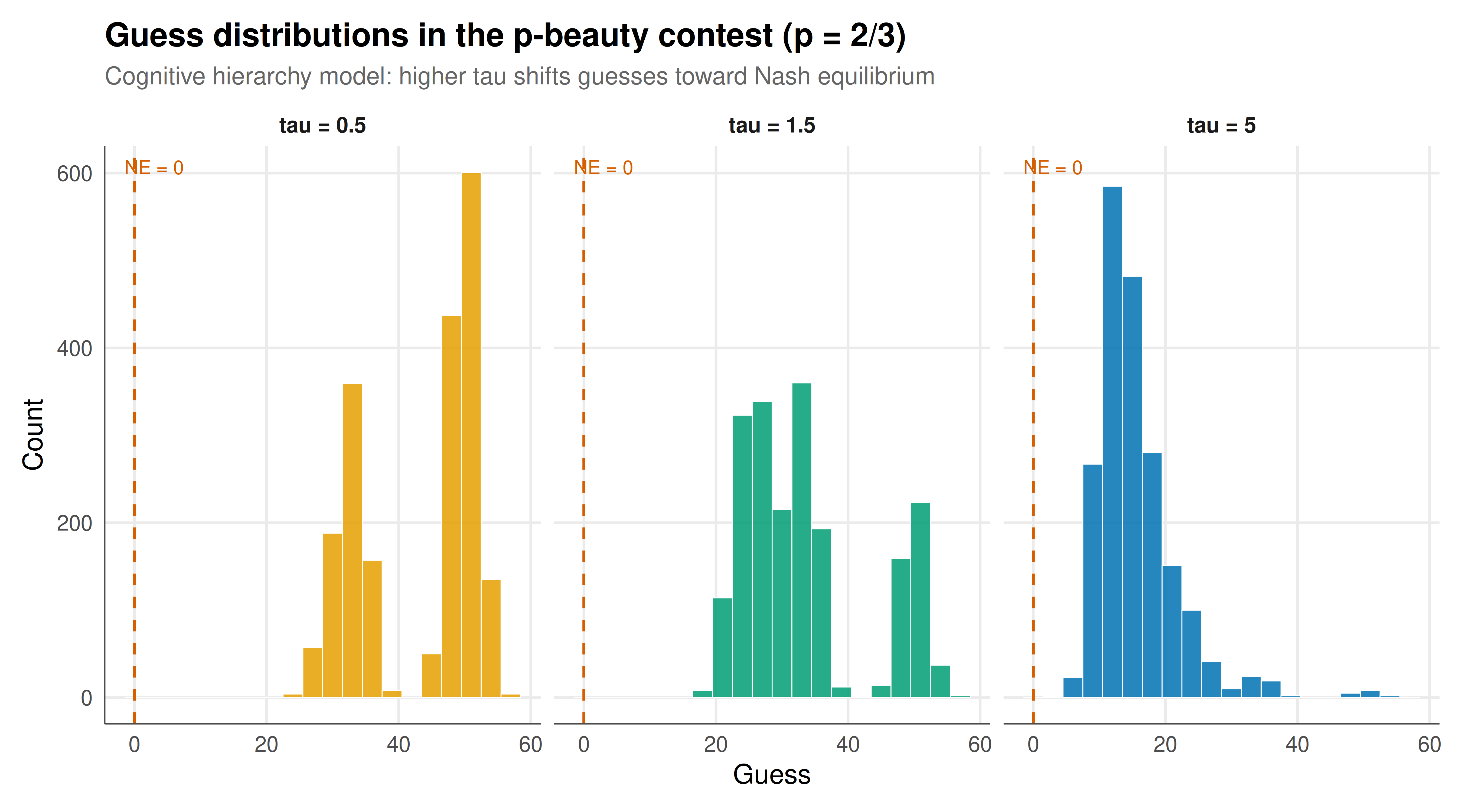
#| label: fig-ch-guess-distributions
#| fig-cap: "Figure 1. Distribution of guesses in the p-beauty contest (p=2/3) under the cognitive hierarchy model for three values of tau. With low tau (0.5), most players are L0 or L1 and guesses cluster around 33-50. With empirically calibrated tau (1.5), guesses spread across 15-50 with a peak near 25-35. With high tau (5.0), the distribution shifts toward lower guesses, approaching Nash equilibrium. Each histogram is based on 2000 simulated players. The red dashed line marks the Nash equilibrium at 0. Okabe-Ito palette."
#| dev: [png, pdf]
#| fig-width: 9
#| fig-height: 5
#| dpi: 300
set.seed(123)
tau_values <- c(0.5, 1.5, 5.0)
sim_all <- lapply(tau_values, function(tau) {
  sim <- simulate_ch_population(2000, tau)
  sim$tau_label <- paste0("tau = ", tau)
  sim
}) |> bind_rows() |>
  mutate(tau_label = factor(tau_label, levels = paste0("tau = ", tau_values)))

p_static <- ggplot(sim_all, aes(x = guess, fill = tau_label)) +
  geom_histogram(binwidth = 3, alpha = 0.85, color = "white", linewidth = 0.2) +
  geom_vline(xintercept = 0, linetype = "dashed", color = "#D55E00", linewidth = 0.6) +
  annotate("text", x = 3, y = Inf, label = "NE = 0", vjust = 2,
           color = "#D55E00", size = 3) +
  facet_wrap(~tau_label, ncol = 3) +
  scale_fill_manual(values = okabe_ito[c(1, 3, 5)], guide = "none") +
  labs(title = "Guess distributions in the p-beauty contest (p = 2/3)",
       subtitle = "Cognitive hierarchy model: higher tau shifts guesses toward Nash equilibrium",
       x = "Guess", y = "Count") +
  theme_publication() +
  theme(strip.text = element_text(face = "bold"))

p_static
```
## Interactive figure
```{r}
#| label: fig-convergence-interactive
# Aggregate guess as function of tau
tau_seq <- seq(0.1, 15, by = 0.1)
convergence_data <- tibble(
  tau = tau_seq,
  aggregate_guess = sapply(tau_seq, aggregate_guess)
) |>
  mutate(text = paste0("tau = ", round(tau, 1),
                       "\nAggregate guess = ", round(aggregate_guess, 2)))

# Also show level-k sequence
lk_data <- tibble(
  level = 0:10,
  guess = lk_guesses[1:11]
) |>
  mutate(text = paste0("Level ", level, "\nGuess = ", round(guess, 2)))

# Combine into a two-panel interactive plot
p_conv <- ggplot(convergence_data, aes(x = tau, y = aggregate_guess, text = text)) +
  geom_line(linewidth = 1, color = okabe_ito[5]) +
  geom_hline(yintercept = 0, linetype = "dashed", color = "grey50") +
  geom_point(data = tibble(tau = 1.5, aggregate_guess = aggregate_guess(1.5),
                            text = paste0("Empirical tau = 1.5\nGuess = ",
                                          round(aggregate_guess(1.5), 2))),
             color = okabe_ito[6], size = 3) +
  labs(title = "CH aggregate prediction converges to NE as tau increases",
       subtitle = "Orange dot = empirically estimated tau (1.5)",
       x = expression("Mean thinking depth " * tau),
       y = "Aggregate predicted guess") +
  theme_publication()

ggplotly(p_conv, tooltip = "text") |>
  config(displaylogo = FALSE, modeBarButtonsToRemove = c("select2d", "lasso2d"))
```
## Interpretation
The level-k and cognitive hierarchy models provide a structured explanation for the persistent gap between Nash equilibrium predictions and observed behaviour in experiments. In the p-beauty contest with $p = 2/3$, Nash equilibrium predicts everyone guesses 0, but the cognitive hierarchy model with the empirically calibrated $\tau = 1.5$ predicts an aggregate guess around 27 --- remarkably close to the 20--35 range typically observed in experiments with first-time players. The Poisson distribution at $\tau = 1.5$ implies that about 22% of players are L0, 34% are L1, 25% are L2, and the remaining 19% are at higher levels. This matches the common experimental finding that the modal type is L1, with substantial fractions at L0 and L2, and few players reasoning beyond L3.
The convergence to Nash equilibrium as $\tau \to \infty$ is theoretically reassuring: Nash equilibrium is the limiting case of the cognitive hierarchy when all players are infinitely sophisticated. But for realistic finite $\tau$, the model makes sharply different predictions. A key insight from @camerer_ho_chong_2004 is that the CH model, calibrated on one game, can predict behaviour across very different games using the same $\tau$ --- suggesting that strategic sophistication is partially a stable individual trait rather than being entirely game-specific.
The practical implications are significant for mechanism design and market design: if you assume Nash equilibrium behaviour when designing an institution, you may get systematically different outcomes because real agents reason at finite depth. Auction designers, platform architects, and policy-makers should consider how their mechanisms perform not just at Nash equilibrium but across the distribution of reasoning depths they expect in their population.
## Extensions & related tutorials
- [Mixed-strategy Nash equilibrium](../../foundations/nash-equilibrium-mixed/) --- the standard equilibrium concept that level-k reasoning approximates.
- [Ultimatum game and fairness](../ultimatum-game-fairness/) --- another setting where bounded rationality and fairness norms drive behaviour away from Nash predictions.
- [Public goods with punishment](../public-goods-punishment/) --- strategic interaction where beliefs about others' reasoning depth matter.
- [Penalty kicks as minimax game](../../real-world-data-applications/penalty-kicks-minimax/) --- testing game-theoretic predictions against real-world data.
- [Prospect theory and reference dependence](../../decision-theory/prospect-theory-reference-dependence/) --- another behavioral departure from standard rationality.
## References
::: {#refs}
:::