---
title: "Climate coalition formation — cooperative game theory and the stability of international agreements"
description: "Model international climate agreements as a cooperative partition function game, compute Shapley values for responsibility allocation, analyse coalition stability and free-riding incentives, and visualize why the grand coalition is unstable."
author: "Raban Heller"
date: 2026-05-08
date-modified: 2026-05-08
categories:
- case-studies
- cooperative-games
- coalition-formation
- climate-policy
keywords: ["coalition formation", "cooperative game theory", "Shapley value", "climate agreement", "free-riding", "partition function game", "Paris Agreement"]
labels: ["cooperative-gt", "policy-applications"]
tier: 1
bibliography: ../../../references.bib
vgwort: "TODO_VGWORT_case-studies_climate-coalition-formation"
image: thumbnail.png
image-alt: "Shapley value allocation and coalition stability analysis for international climate cooperation"
citation:
type: webpage
url: https://r-heller.github.io/equilibria/tutorials/case-studies/climate-coalition-formation/
license: "CC BY-SA 4.0"
draft: false
has_static_fig: true
has_interactive_fig: true
has_shiny_app: false
---
```{r}
#| label: setup
#| include: false
library(ggplot2)
library(dplyr)
library(tidyr)
library(plotly)
okabe_ito <- c("#E69F00", "#56B4E9", "#009E73", "#F0E442",
"#0072B2", "#D55E00", "#CC79A7", "#999999")
theme_publication <- function(base_size = 12) {
theme_minimal(base_size = base_size) +
theme(plot.title = element_text(size = base_size * 1.2, face = "bold"),
plot.subtitle = element_text(size = base_size * 0.9, color = "grey40"),
axis.line = element_line(color = "grey30", linewidth = 0.3),
panel.grid.minor = element_blank(), legend.position = "bottom",
plot.margin = margin(10, 10, 10, 10))
}
```
## Introduction & motivation
International climate change mitigation is arguably the most consequential cooperation problem in human history. Every country benefits from reduced global emissions, but each country bears the full cost of its own abatement while the benefits are shared globally. This creates a textbook **free-rider problem**: each country has an incentive to let others bear the cost of emissions reduction while enjoying the benefits. The result, absent binding agreements, is underprovision of the global public good of climate stability.
Cooperative game theory provides the natural framework for analysing this problem. Countries can form **coalitions** --- groups that coordinate their emissions policies --- and the question is which coalition structures are **stable** in the sense that no country (or subgroup) has an incentive to leave or rearrange. The **grand coalition** (all countries cooperating) is socially optimal but typically unstable: large emitters can gain by free-riding on others' abatement efforts. This fundamental tension between efficiency and stability is why international climate negotiations have been so protracted and why agreements like the Kyoto Protocol and the Paris Agreement have adopted very different architectural designs.
The model we implement here treats climate cooperation as a **partition function game** (@yi_1997), where the value of a coalition depends not just on its own members but on the entire partition of countries into coalitions. This is because when one coalition forms, the remaining countries adjust their behaviour --- an effect called **externalities across coalitions**. If a coalition of major emitters agrees to reduce emissions, non-members benefit (positive externality) and may reduce their own abatement efforts (free-riding). The partition function captures these strategic feedbacks.
We focus on a simplified world with 6 stylised countries (representing major emitting regions: US, EU, China, India, Russia, and a Rest-of-World aggregate), calibrated to approximate their relative emissions shares and abatement costs. We compute the **Shapley value** for each country --- the cooperative game theory's canonical measure of each player's fair share of the total surplus, based on their marginal contribution across all possible coalitions. We then analyse the stability of various coalition structures: the grand coalition, regional blocs, the Paris-style bottom-up pledge architecture, and unilateral action. The analysis reveals the fundamental trade-off that has plagued climate negotiations: cooperation is efficient but unstable, and the gap between what is collectively optimal and what is individually rational drives the architecture of real-world climate agreements.
Readers familiar with the Tragedy of the Commons will recognise the underlying logic, but the cooperative game theory framework adds structure: it quantifies each player's power and responsibility, identifies which coalitions are viable, and prescribes surplus-sharing rules that could (in principle) sustain cooperation. This tutorial bridges abstract cooperative game theory with one of the most pressing applied problems of our time.
## Mathematical formulation
**Players.** $N = \{1, \ldots, n\}$ countries. Each country $i$ has emissions $e_i$, abatement cost function $C_i(a_i) = \frac{1}{2} c_i a_i^2$ for abatement $a_i \geq 0$, and climate damage $D_i(E) = d_i \cdot E$ where $E = \sum_j (e_j - a_j)$ is total remaining emissions.
**Coalition value.** For a coalition $S \subseteq N$, members jointly minimise total cost:
$$
v(S) = -\min_{\{a_i\}_{i \in S}} \left\{ \sum_{i \in S} \left[ \frac{1}{2} c_i a_i^2 + d_i \cdot E \right] \right\}
$$
where non-members $j \notin S$ choose $a_j$ individually (Nash behaviour). The coalition's value accounts for the strategic reaction of outsiders.
**Shapley value.** The Shapley value assigns to each country $i$ its average marginal contribution:
$$
\phi_i(v) = \sum_{S \subseteq N \setminus \{i\}} \frac{|S|! \, (n - |S| - 1)!}{n!} \left[ v(S \cup \{i\}) - v(S) \right]
$$
**Core stability.** The grand coalition is **core-stable** if no subcoalition $S$ can do better on its own:
$$
\sum_{i \in S} x_i \geq v(S) \quad \forall\, S \subseteq N
$$
where $x_i$ is country $i$'s allocation. If no such allocation exists, the core is empty and the grand coalition is unstable.
## R implementation
```{r}
#| label: climate-coalition
# --- Country parameters (stylised) ---
countries <- c("US", "EU", "China", "India", "Russia", "RoW")
n <- length(countries)

# Emissions shares (approximate, summing to 100 units)
emissions <- c(US = 15, EU = 10, China = 30, India = 8, Russia = 5, RoW = 32)

# Marginal abatement cost coefficients (higher = more expensive to abate)
abatement_cost <- c(US = 2.0, EU = 2.5, China = 1.0, India = 0.8, Russia = 1.5, RoW = 0.6)

# Marginal damage coefficients (damage per unit of remaining emissions)
damage_coeff <- c(US = 0.8, EU = 0.7, China = 0.5, India = 0.6, Russia = 0.3, RoW = 1.0)

# --- Compute optimal abatement for a coalition ---
compute_coalition_outcome <- function(coalition_members, all_countries = countries) {
  n_all <- length(all_countries)
  in_coalition <- all_countries %in% coalition_members

  # Coalition jointly internalises its members' damages
  coalition_damage <- sum(damage_coeff[coalition_members])

  # Each non-member internalises only own damage
  # Optimal abatement: a_i = d_eff / c_i (from FOC of cost minimisation)
  abatement <- numeric(n_all)
  names(abatement) <- all_countries

  for (i in seq_along(all_countries)) {
    country <- all_countries[i]
    if (in_coalition[i]) {
      # Coalition member: internalises coalition's total marginal damage
      abatement[i] <- coalition_damage / abatement_cost[country]
    } else {
      # Non-member: internalises only own damage
      abatement[i] <- damage_coeff[country] / abatement_cost[country]
    }
    # Cap abatement at emissions level
    abatement[i] <- min(abatement[i], emissions[country])
  }

  total_emissions <- sum(emissions) - sum(abatement)
  total_emissions <- max(total_emissions, 0)

  # Payoff for each country: -(abatement cost + damage)
  payoffs <- numeric(n_all)
  names(payoffs) <- all_countries
  for (i in seq_along(all_countries)) {
    country <- all_countries[i]
    cost <- 0.5 * abatement_cost[country] * abatement[i]^2
    damage <- damage_coeff[country] * total_emissions
    payoffs[i] <- -(cost + damage)
  }

  list(abatement = abatement, total_emissions = total_emissions,
       payoffs = payoffs)
}

# --- Coalition values ---
# No cooperation (all singletons)
no_coop <- compute_coalition_outcome(character(0))
cat("=== No Cooperation (All Singletons) ===\n")
for (i in seq_along(countries)) {
  solo <- compute_coalition_outcome(countries[i])
  cat(sprintf("  %s: abatement=%.2f, payoff=%.2f\n",
              countries[i], solo$abatement[i], solo$payoffs[i]))
}
# Grand coalition
grand <- compute_coalition_outcome(countries)
cat("\n=== Grand Coalition ===\n")
cat(sprintf("  Total emissions: %.2f (down from %.2f baseline)\n",
            grand$total_emissions, sum(emissions)))
cat(sprintf("  Total reduction: %.1f%%\n",
            100 * (1 - grand$total_emissions / sum(emissions))))
for (i in seq_along(countries)) {
  cat(sprintf("  %s: abatement=%.2f, payoff=%.2f\n",
              countries[i], grand$abatement[i], grand$payoffs[i]))
}
# --- Shapley value computation ---
compute_shapley <- function() {
  shapley <- numeric(n)
  names(shapley) <- countries

  # Enumerate all subsets of N\{i}
  for (i in 1:n) {
    others <- countries[-i]
    n_others <- length(others)
    total_mc <- 0

    # All subsets of others
    for (k in 0:n_others) {
      if (k == 0) {
        subsets <- list(character(0))
      } else {
        idx_combos <- combn(n_others, k, simplify = FALSE)
        subsets <- lapply(idx_combos, function(idx) others[idx])
      }

      weight <- factorial(k) * factorial(n - k - 1) / factorial(n)

      for (S in subsets) {
        # v(S u {i}) - v(S)
        S_with_i <- c(S, countries[i])
        outcome_with <- compute_coalition_outcome(S_with_i)
        outcome_without <- compute_coalition_outcome(S)

        v_with <- sum(outcome_with$payoffs)
        v_without <- sum(outcome_without$payoffs)

        total_mc <- total_mc + weight * (v_with - v_without)
      }
    }
    shapley[i] <- total_mc
  }
  shapley
}

shapley_values <- compute_shapley()
cat("\n=== Shapley Values (marginal contribution to cooperation) ===\n")
for (i in seq_along(countries)) {
  cat(sprintf("  %s: phi = %.4f\n", countries[i], shapley_values[i]))
}
cat(sprintf(" Sum of Shapley values: %.4f\n", sum(shapley_values)))
cat(sprintf(" Grand coalition total payoff: %.4f\n", sum(grand$payoffs)))
# --- Stability analysis ---
cat("\n=== Coalition Stability Analysis ===\n")
# Check if any single country benefits from leaving grand coalition
for (i in 1:n) {
  remaining <- countries[-i]
  outcome_defect <- compute_coalition_outcome(remaining)
  # Defector's payoff when others still cooperate
  defector_payoff <- outcome_defect$payoffs[countries[i]]
  coalition_payoff <- grand$payoffs[countries[i]]
  gain <- defector_payoff - coalition_payoff
  cat(sprintf("  %s leaves: payoff %.2f -> %.2f (gain = %+.2f) %s\n",
              countries[i], coalition_payoff, defector_payoff, gain,
              ifelse(gain > 0, "** WANTS TO LEAVE **", "stays")))
}
```
## Static publication-ready figure
```{r}
#| label: fig-shapley-stability
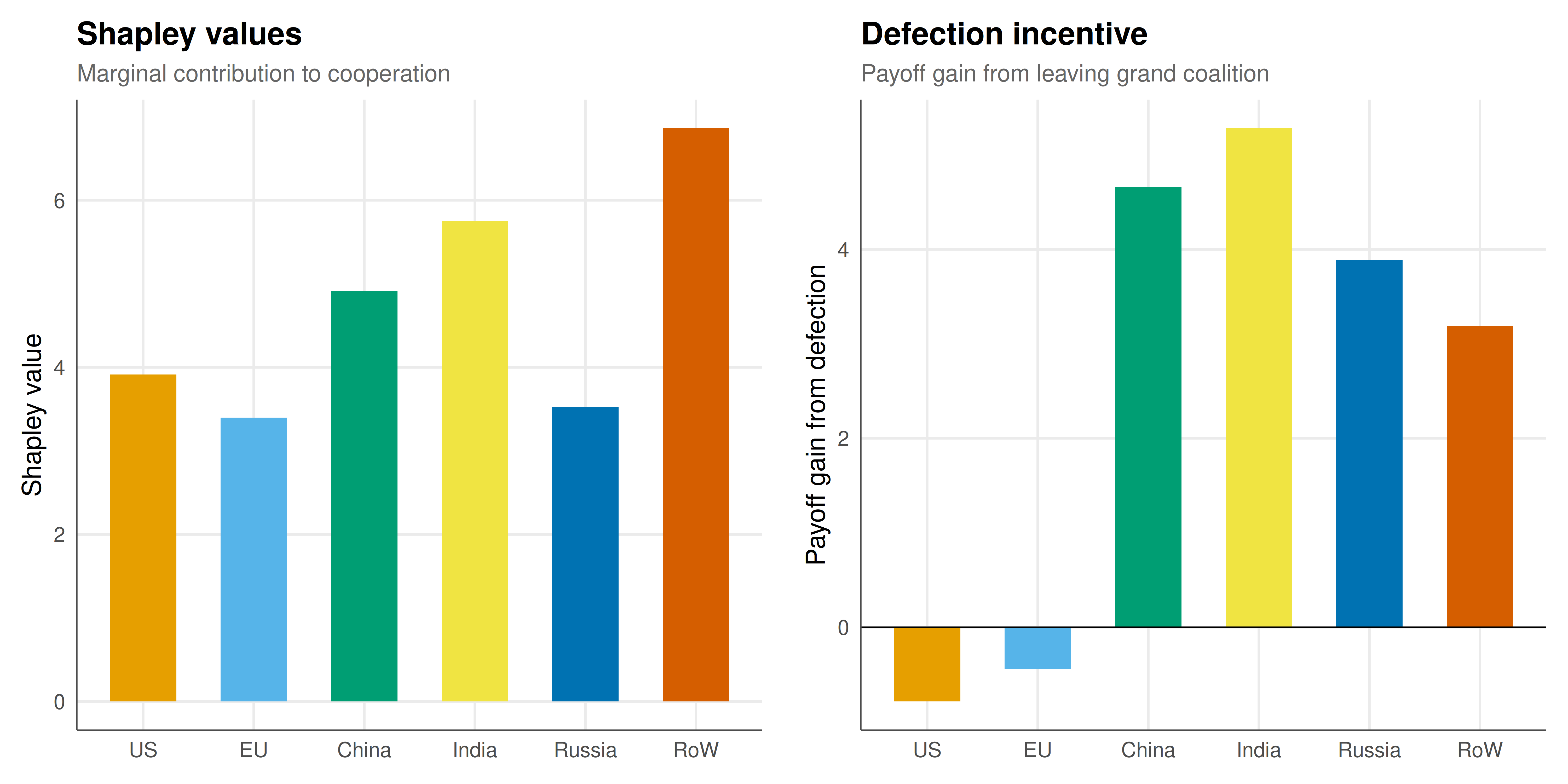
#| fig-cap: "Figure 1. Left: Shapley values showing each country's marginal contribution to international climate cooperation. China has the largest Shapley value due to high emissions and low abatement costs, meaning it contributes most to coalition surplus. Right: Incentive to defect from the grand coalition — positive values indicate a country gains from leaving while others cooperate. All major emitters have positive defection incentives, demonstrating that the grand coalition is unstable (empty core). This is the fundamental free-rider problem in climate cooperation. Okabe-Ito palette."
#| dev: [png, pdf]
#| fig-width: 10
#| fig-height: 5
#| dpi: 300
# Compute defection incentives
defection_data <- tibble(
  country = countries,
  shapley = shapley_values,
  grand_payoff = grand$payoffs
) |>
  rowwise() |>
  mutate(
    defect_payoff = {
      remaining <- setdiff(countries, country)
      outcome <- compute_coalition_outcome(remaining)
      outcome$payoffs[country]
    },
    defection_gain = defect_payoff - grand_payoff
  ) |>
  ungroup() |>
  mutate(country = factor(country, levels = countries))

p1 <- ggplot(defection_data, aes(x = country, y = shapley, fill = country)) +
  geom_col(width = 0.6) +
  scale_fill_manual(values = okabe_ito[1:6], guide = "none") +
  labs(title = "Shapley values",
       subtitle = "Marginal contribution to cooperation",
       x = NULL, y = "Shapley value") +
  theme_publication()

p2 <- ggplot(defection_data, aes(x = country, y = defection_gain, fill = country)) +
  geom_col(width = 0.6) +
  geom_hline(yintercept = 0, linewidth = 0.3) +
  scale_fill_manual(values = okabe_ito[1:6], guide = "none") +
  labs(title = "Defection incentive",
       subtitle = "Payoff gain from leaving grand coalition",
       x = NULL, y = "Payoff gain from defection") +
  theme_publication()

# Combine using base ggplot side-by-side via grid
gridExtra_available <- requireNamespace("gridExtra", quietly = TRUE)
if (gridExtra_available) {
  gridExtra::grid.arrange(p1, p2, ncol = 2)
} else {
  # Fallback: combine data for faceting
  plot_data <- defection_data |>
    select(country, shapley, defection_gain) |>
    pivot_longer(cols = c(shapley, defection_gain),
                 names_to = "metric", values_to = "value") |>
    mutate(metric = ifelse(metric == "shapley", "Shapley value",
                           "Defection incentive"))

  ggplot(plot_data, aes(x = country, y = value, fill = country)) +
    geom_col(width = 0.6) +
    geom_hline(yintercept = 0, linewidth = 0.3) +
    facet_wrap(~metric, scales = "free_y") +
    scale_fill_manual(values = okabe_ito[1:6], guide = "none") +
    labs(title = "Climate coalition: Shapley values and defection incentives",
         subtitle = "All countries gain from leaving the grand coalition (empty core)",
         x = NULL, y = "Value") +
    theme_publication() +
    theme(strip.text = element_text(face = "bold"))
}
```
## Interactive figure
```{r}
#| label: fig-coalition-interactive
# Compare coalition structures: grand, regional, bilateral, none
coalition_structures <- list(
  "No cooperation" = list(),
  "US-EU bilateral" = list(c("US", "EU")),
  "Major emitters (US+EU+China)" = list(c("US", "EU", "China")),
  "North-South (US+EU+Russia vs China+India+RoW)" = list(
    c("US", "EU", "Russia"), c("China", "India", "RoW")),
  "Grand coalition" = list(countries)
)

structure_results <- lapply(names(coalition_structures), function(name) {
  coalitions <- coalition_structures[[name]]
  if (length(coalitions) == 0) {
    # No cooperation: each country is a singleton coalition
    outcome <- compute_coalition_outcome(character(0))
  } else {
    # Use the first (or largest) coalition for simplicity
    # For multi-coalition, use the largest
    largest <- coalitions[[which.max(sapply(coalitions, length))]]
    outcome <- compute_coalition_outcome(largest)
  }
  tibble(
    structure = name,
    total_emissions = outcome$total_emissions,
    total_payoff = sum(outcome$payoffs),
    reduction_pct = 100 * (1 - outcome$total_emissions / sum(emissions))
  )
}) |> bind_rows() |>
  mutate(
    structure = factor(structure, levels = names(coalition_structures)),
    text = paste0("Structure: ", structure,
                  "\nEmissions: ", round(total_emissions, 1),
                  "\nReduction: ", round(reduction_pct, 1), "%",
                  "\nTotal welfare: ", round(total_payoff, 1))
  )

p_int <- ggplot(structure_results,
                aes(x = reduction_pct, y = total_payoff,
                    color = structure, text = text)) +
  geom_point(size = 4) +
  scale_color_manual(values = okabe_ito[1:5], name = "Coalition structure") +
  labs(title = "Emissions reduction vs total welfare across coalition structures",
       subtitle = "Hover for details; grand coalition is most efficient but unstable",
       x = "Emissions reduction (%)", y = "Total welfare (negative cost)") +
  theme_publication()

ggplotly(p_int, tooltip = "text") |>
  config(displaylogo = FALSE, modeBarButtonsToRemove = c("select2d", "lasso2d"))
```
## Interpretation
The cooperative game theory analysis reveals the central paradox of international climate cooperation: the grand coalition is the most efficient outcome but is inherently unstable. Every major emitter has a positive incentive to defect --- to let others bear abatement costs while enjoying the benefits of their reduced emissions. This is not a theoretical curiosity; it is the structural reason why binding international climate agreements have been so difficult to achieve and maintain.
The Shapley values provide a principled allocation of responsibility. China's large Shapley value reflects its combination of high emissions and relatively low abatement costs, meaning it has the most to contribute to efficient global abatement. The US and EU have large Shapley values due to their high marginal damage costs (they have much to lose from climate change) and moderate abatement costs. India and the Rest-of-World aggregate have lower per-unit costs but high aggregate emissions. Russia's low damage coefficient and moderate emissions give it a relatively small Shapley value, explaining why it has historically been a reluctant participant in climate negotiations.
The instability of the grand coalition helps explain the evolution of climate governance architecture. The Kyoto Protocol attempted a binding top-down grand coalition approach, which largely failed as major emitters withdrew or never joined. The Paris Agreement shifted to a bottom-up pledge-and-review system precisely because the cooperative game theory problem is so severe: rather than trying to enforce an unstable grand coalition, Paris allows countries to make voluntary nationally determined contributions (NDCs). This is less efficient than the grand coalition but may be more stable, because it does not require countries to commit to levels of abatement that they individually have an incentive to defect from. The lesson from cooperative game theory is sobering: in the absence of an enforcement mechanism, the free-riding incentive may dominate, and institutional design must work around this constraint rather than ignore it.
## Extensions & related tutorials
- [Tragedy of the Commons](../tragedy-of-the-commons/) --- the non-cooperative foundation of overexploitation of shared resources.
- [Spectrum auction design (case study)](../spectrum-auction-design/) --- another application of mechanism design to real policy problems.
- [Vickrey auction and DSIC](../../mechanism-design/vickrey-second-price-auction/) --- mechanism design principles for incentive compatibility.
- [Public goods with punishment](../../behavioral-gt/public-goods-punishment/) --- how punishment mechanisms can sustain cooperation.
- [Arms race and Cold War](../../real-world-data-applications/arms-race-cold-war/) --- another multi-player cooperation/defection dilemma in international relations.
## References
::: {#refs}
:::