---
title: "The arms race as iterated Prisoner's Dilemma — a Cold War analysis"
description: "Model the US-Soviet nuclear arms race as an iterated Prisoner's Dilemma in R, simulate strategy profiles including MAD, compare with stylised historical spending patterns, and connect to the folk theorem."
author: "Raban Heller"
date: 2026-05-08
date-modified: 2026-05-08
categories:
- real-world-data-applications
- arms-race
- prisoners-dilemma
- cold-war
keywords: ["arms race", "Cold War", "iterated Prisoner's Dilemma", "mutually assured destruction", "nuclear weapons", "folk theorem", "tit-for-tat"]
labels: ["applied-game-theory", "historical-applications"]
tier: 1
bibliography: ../../../references.bib
vgwort: "TODO_VGWORT_real-world-data-applications_arms-race-cold-war"
image: thumbnail.png
image-alt: "Simulated arms spending trajectories for US and Soviet Union under different strategic profiles"
citation:
type: webpage
url: https://r-heller.github.io/equilibria/tutorials/real-world-data-applications/arms-race-cold-war/
license: "CC BY-SA 4.0"
draft: false
has_static_fig: true
has_interactive_fig: true
has_shiny_app: false
---
```{r}
#| label: setup
#| include: false
library(ggplot2)
library(dplyr)
library(tidyr)
library(plotly)
okabe_ito <- c("#E69F00", "#56B4E9", "#009E73", "#F0E442",
"#0072B2", "#D55E00", "#CC79A7", "#999999")
theme_publication <- function(base_size = 12) {
theme_minimal(base_size = base_size) +
theme(
plot.title = element_text(size = base_size * 1.2, face = "bold"),
plot.subtitle = element_text(size = base_size * 0.9, color = "grey40"),
axis.line = element_line(color = "grey30", linewidth = 0.3),
panel.grid.minor = element_blank(),
legend.position = "bottom",
plot.margin = margin(10, 10, 10, 10)
)
}
```
## Introduction & motivation
The nuclear arms race between the United States and the Soviet Union, spanning from the end of World War II in 1945 to the dissolution of the Soviet Union in 1991, represents one of the most consequential strategic interactions in human history. At its peak, the two superpowers possessed over 60,000 nuclear warheads combined -- enough to destroy human civilisation many times over. Both sides recognised that this mutual buildup was enormously costly and dangerous, yet neither could unilaterally disarm without exposing itself to catastrophic vulnerability. This is precisely the structure of the **Prisoner's Dilemma**: mutual cooperation (disarmament) is collectively optimal, mutual defection (arming) is collectively inferior, but each side has an individual incentive to arm regardless of what the other does.
The Cold War arms race is not merely a historical curiosity -- it is a canonical case study for understanding how repeated strategic interaction can sustain cooperation (or fail to do so) and how the structure of payoffs shapes long-run outcomes. The early phase (1945-1962) saw rapid escalation as both sides built nuclear arsenals and delivery systems. The Cuban Missile Crisis of 1962 brought the world to the brink of nuclear war and fundamentally altered the strategic calculus by making the consequences of defection catastrophically clear. The subsequent period saw the emergence of **mutually assured destruction (MAD)** as an explicit strategic doctrine: both sides maintained second-strike capability, ensuring that any nuclear first strike would be met with devastating retaliation. MAD effectively changed the payoff structure from a standard Prisoner's Dilemma to a game where mutual defection (nuclear war) yields the worst possible outcome for both players, potentially making cooperation self-enforcing.
This tutorial models the arms race as an **iterated Prisoner's Dilemma (IPD)** with payoffs calibrated to Cold War incentives. We simulate different strategic profiles -- both arm (the historical outcome for much of the Cold War), tit-for-tat reciprocity (which approximates the detente periods), and cooperation attempts (arms control treaties). We show how MAD altered the game by introducing catastrophic punishment for aggression, effectively creating the conditions for the folk theorem to apply: when the shadow of the future is long enough and punishment is severe enough, cooperation becomes sustainable. We compare these simulations with stylised patterns of historical military spending and draw lessons about the conditions under which arms control succeeds or fails. The analysis connects the historical narrative to formal game-theoretic concepts, demonstrating how abstract theory illuminates one of the defining conflicts of the twentieth century.
## Mathematical formulation
Each period $t = 1, 2, \ldots, T$, the two superpowers (US = Player 1, USSR = Player 2) simultaneously choose **Arm** (A) or **Disarm** (D). The stage-game payoffs:
$$
\begin{array}{c|cc}
& \text{Disarm} & \text{Arm} \\ \hline
\text{Disarm} & R, R & S, T \\
\text{Arm} & T, S & P, P
\end{array}
$$
with the Prisoner's Dilemma ordering $T > R > P > S$ and $2R > T + S$.
**Pre-MAD calibration** (1945-1962): $T = 5$ (unilateral military advantage), $R = 3$ (mutual disarmament), $P = 1$ (costly arms race), $S = 0$ (unilateral vulnerability).
**Post-MAD calibration** (1962-1991): MAD introduces catastrophic mutual destruction risk. We model this by changing the mutual defection payoff to reflect the possibility of nuclear war: $P_{\text{MAD}} = -10$ (both arm, risk of annihilation), while maintaining $T = 5, R = 3, S = 0$. Under MAD, the game is no longer a standard PD because $P_{\text{MAD}} < S$ -- mutual arming is now the *worst* outcome, creating a Chicken-like structure.
**Iterated game**: With discount factor $\delta$, the total payoff is:
$$
U_i = \sum_{t=1}^{T} \delta^{t-1} u_i(a_1^t, a_2^t)
$$
**Folk theorem**: For $\delta$ sufficiently close to 1, any feasible individually rational payoff vector can be sustained as a subgame-perfect equilibrium of the infinitely repeated game. For the pre-MAD PD, the minimum discount factor for sustaining cooperation via grim trigger is:
$$
\delta^* = \frac{T - R}{T - P} = \frac{5 - 3}{5 - 1} = 0.5
$$
## R implementation
```{r}
#| label: arms-race-simulation
# Define stage-game payoffs
payoffs_pre_mad <- list(T = 5, R = 3, P = 1, S = 0)
payoffs_mad <- list(T = 5, R = 3, P = -10, S = 0)

# Strategy functions: return "A" (arm) or "D" (disarm) given history
strategy_always_arm <- function(history, player) "A"
strategy_always_disarm <- function(history, player) "D"

strategy_tit_for_tat <- function(history, player) {
  if (nrow(history) == 0) return("D")  # Start cooperating
  opponent <- ifelse(player == 1, 2, 1)
  history[nrow(history), opponent]  # Copy opponent's last action
}

strategy_grim_trigger <- function(history, player) {
  if (nrow(history) == 0) return("D")
  opponent <- ifelse(player == 1, 2, 1)
  if (any(history[, opponent] == "A")) return("A")  # Punish forever
  "D"
}

# Simulate iterated game
simulate_ipd <- function(strat1, strat2, payoffs, T_periods = 46, delta = 0.95) {
  history <- data.frame(P1 = character(0), P2 = character(0),
                         stringsAsFactors = FALSE)
  results <- tibble(
    period = integer(), action1 = character(), action2 = character(),
    payoff1 = numeric(), payoff2 = numeric(),
    cum_payoff1 = numeric(), cum_payoff2 = numeric()
  )

  cum1 <- 0; cum2 <- 0
  for (t in 1:T_periods) {
    a1 <- strat1(history, 1)
    a2 <- strat2(history, 2)
    history <- rbind(history, data.frame(P1 = a1, P2 = a2, stringsAsFactors = FALSE))

    # Look up payoffs
    if (a1 == "D" && a2 == "D") {
      p1 <- payoffs$R; p2 <- payoffs$R
    } else if (a1 == "A" && a2 == "D") {
      p1 <- payoffs$T; p2 <- payoffs$S
    } else if (a1 == "D" && a2 == "A") {
      p1 <- payoffs$S; p2 <- payoffs$T
    } else {
      p1 <- payoffs$P; p2 <- payoffs$P
    }

    cum1 <- cum1 + delta^(t-1) * p1
    cum2 <- cum2 + delta^(t-1) * p2

    results <- bind_rows(results, tibble(
      period = t, action1 = a1, action2 = a2,
      payoff1 = p1, payoff2 = p2,
      cum_payoff1 = cum1, cum_payoff2 = cum2
    ))
  }
  results
}

# Scenario 1: Both always arm (historical Cold War approximation)
cat("=== Scenario 1: Both Always Arm (pre-MAD) ===\n")
sim1 <- simulate_ipd(strategy_always_arm, strategy_always_arm, payoffs_pre_mad)
cat(sprintf("Final cumulative payoffs: US = %.1f, USSR = %.1f\n",
            tail(sim1$cum_payoff1, 1), tail(sim1$cum_payoff2, 1)))
cat(sprintf("Per-period: both get P = %d\n", payoffs_pre_mad$P))
# Scenario 2: Tit-for-Tat vs Tit-for-Tat (detente)
cat("\n=== Scenario 2: Tit-for-Tat vs Tit-for-Tat (detente) ===\n")
sim2 <- simulate_ipd(strategy_tit_for_tat, strategy_tit_for_tat, payoffs_pre_mad)
cat(sprintf("Final cumulative payoffs: US = %.1f, USSR = %.1f\n",
            tail(sim2$cum_payoff1, 1), tail(sim2$cum_payoff2, 1)))
cat(sprintf("Per-period: both get R = %d (sustained cooperation)\n", payoffs_pre_mad$R))
# Scenario 3: Grim trigger vs Grim trigger (arms control treaty)
cat("\n=== Scenario 3: Grim Trigger vs Grim Trigger (arms control) ===\n")
sim3 <- simulate_ipd(strategy_grim_trigger, strategy_grim_trigger, payoffs_pre_mad)
cat(sprintf("Final cumulative payoffs: US = %.1f, USSR = %.1f\n",
            tail(sim3$cum_payoff1, 1), tail(sim3$cum_payoff2, 1)))
# Scenario 4: MAD payoffs with always arm
cat("\n=== Scenario 4: Both Always Arm under MAD ===\n")
sim4 <- simulate_ipd(strategy_always_arm, strategy_always_arm, payoffs_mad)
cat(sprintf("Final cumulative payoffs: US = %.1f, USSR = %.1f\n",
            tail(sim4$cum_payoff1, 1), tail(sim4$cum_payoff2, 1)))
cat(sprintf("Per-period: both get P_MAD = %d (catastrophic)\n", payoffs_mad$P))
# Folk theorem: minimum discount factor
cat("\n=== Folk Theorem: Minimum Discount Factor for Cooperation ===\n")
delta_star_pre <- (payoffs_pre_mad$T - payoffs_pre_mad$R) /
                  (payoffs_pre_mad$T - payoffs_pre_mad$P)
delta_star_mad <- (payoffs_mad$T - payoffs_mad$R) /
                  (payoffs_mad$T - payoffs_mad$P)
cat(sprintf("Pre-MAD: delta* = %.3f (cooperation requires moderate patience)\n", delta_star_pre))
cat(sprintf("Post-MAD: delta* = %.3f (MAD makes cooperation much easier to sustain)\n", delta_star_mad))
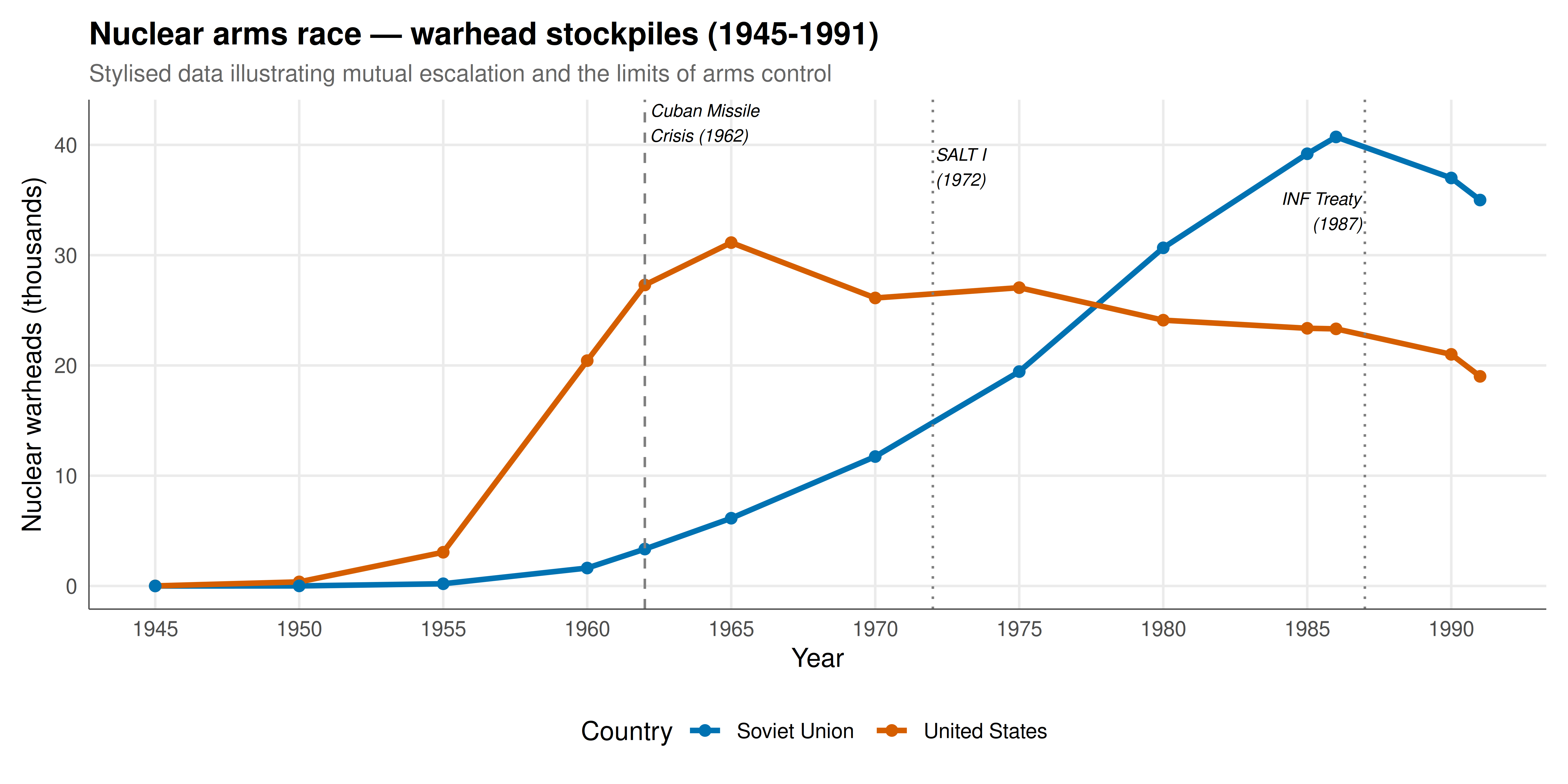
# Stylised historical data: nuclear warhead counts
cat("\n=== Stylised Nuclear Warhead Counts ===\n")
warhead_data <- tibble(
  year = c(1945, 1950, 1955, 1960, 1962, 1965, 1970, 1975,
           1980, 1985, 1986, 1990, 1991),
  us_warheads = c(6, 369, 3057, 20434, 27297, 31139, 26119, 27052,
                  24104, 23368, 23317, 21004, 19008),
  ussr_warheads = c(0, 5, 200, 1627, 3346, 6144, 11736, 19443,
                    30665, 39197, 40723, 37000, 35000)
)
cat("Year | US warheads | USSR warheads\n")
for (i in 1:nrow(warhead_data)) {
  cat(sprintf("%d | %7d     | %7d\n",
              warhead_data$year[i], warhead_data$us_warheads[i],
              warhead_data$ussr_warheads[i]))
}
```
## Static publication-ready figure
```{r}
#| label: fig-arms-race-history
#| fig-cap: "Figure 1. Stylised nuclear warhead counts for the US and Soviet Union (1945-1991) alongside key strategic milestones. The rapid buildup phase (1945-1965) reflects mutual defection in the arms race PD. The Cuban Missile Crisis (1962) marks the emergence of MAD doctrine. The post-SALT stabilisation (1972 onwards) shows the effect of arms control treaties as imperfect cooperation mechanisms. Both sides accumulated far beyond any military necessity, illustrating the waste inherent in Prisoner's Dilemma dynamics. Okabe-Ito palette."
#| dev: [png, pdf]
#| fig-width: 10
#| fig-height: 5
#| dpi: 300
warhead_long <- warhead_data |>
  pivot_longer(cols = c(us_warheads, ussr_warheads),
               names_to = "country", values_to = "warheads") |>
  mutate(country = ifelse(country == "us_warheads", "United States", "Soviet Union"))

p_history <- ggplot(warhead_long, aes(x = year, y = warheads / 1000,
                                       color = country)) +
  geom_line(linewidth = 1.2) +
  geom_point(size = 2) +
  # Key events
  geom_vline(xintercept = 1962, linetype = "dashed", color = "grey50") +
  annotate("text", x = 1962, y = 42, label = "Cuban Missile\nCrisis (1962)",
           size = 2.8, hjust = -0.05, fontface = "italic") +
  geom_vline(xintercept = 1972, linetype = "dotted", color = "grey50") +
  annotate("text", x = 1972, y = 38, label = "SALT I\n(1972)",
           size = 2.8, hjust = -0.05, fontface = "italic") +
  geom_vline(xintercept = 1987, linetype = "dotted", color = "grey50") +
  annotate("text", x = 1987, y = 34, label = "INF Treaty\n(1987)",
           size = 2.8, hjust = 1.05, fontface = "italic") +
  scale_color_manual(values = okabe_ito[c(5, 6)], name = "Country") +
  scale_x_continuous(breaks = seq(1945, 1991, by = 5)) +
  labs(
    title = "Nuclear arms race — warhead stockpiles (1945-1991)",
    subtitle = "Stylised data illustrating mutual escalation and the limits of arms control",
    x = "Year", y = "Nuclear warheads (thousands)"
  ) +
  theme_publication()

p_history
```
## Interactive figure
```{r}
#| label: fig-arms-race-scenarios
# Compare cumulative payoffs across strategic scenarios
scenarios <- bind_rows(
  sim1 |> mutate(scenario = "Both Arm (pre-MAD)"),
  sim2 |> mutate(scenario = "Tit-for-Tat (detente)"),
  sim3 |> mutate(scenario = "Grim Trigger (arms control)"),
  sim4 |> mutate(scenario = "Both Arm (MAD)")
)

# Map periods to approximate years (1945-1991)
scenarios <- scenarios |>
  mutate(year = 1945 + period - 1)

scenario_long <- scenarios |>
  select(year, scenario, cum_payoff1, cum_payoff2) |>
  pivot_longer(cols = c(cum_payoff1, cum_payoff2),
               names_to = "player", values_to = "cum_payoff") |>
  mutate(
    player = ifelse(player == "cum_payoff1", "United States", "Soviet Union"),
    text = paste0("Year: ", year,
                  "\n", player,
                  "\nScenario: ", scenario,
                  "\nCumulative payoff: ", round(cum_payoff, 1))
  )

p_scenarios <- ggplot(scenario_long,
                       aes(x = year, y = cum_payoff, color = scenario,
                           linetype = player, text = text)) +
  geom_line(linewidth = 0.9) +
  scale_color_manual(values = okabe_ito[c(6, 3, 2, 7)], name = "Scenario") +
  scale_linetype_manual(values = c("solid", "dashed"), name = "Player") +
  labs(
    title = "Cumulative payoffs under different Cold War strategies",
    subtitle = "Cooperation (TfT, Grim Trigger) vastly outperforms mutual arming",
    x = "Year", y = "Discounted cumulative payoff"
  ) +
  theme_publication()

ggplotly(p_scenarios, tooltip = "text") |>
  config(displaylogo = FALSE,
         modeBarButtonsToRemove = c("select2d", "lasso2d"))
```
## Interpretation
The simulation results illuminate the tragic logic of the Cold War arms race through the lens of iterated game theory. Under the pre-MAD Prisoner's Dilemma payoffs, mutual arming yields each side a per-period payoff of $P = 1$, while mutual disarmament would yield $R = 3$ -- three times as much. Over 46 years of the Cold War, the cumulative cost of the arms race (relative to the cooperative benchmark) is enormous. The tit-for-tat and grim-trigger scenarios demonstrate that sustained cooperation was theoretically possible: with discount factor $\delta = 0.95$ far exceeding the critical threshold $\delta^* = 0.5$, both superpowers were sufficiently patient for cooperation to be sustained as a subgame-perfect equilibrium.
Why, then, did cooperation largely fail? Several factors explain the gap between theory and reality. First, **information asymmetry**: neither side could perfectly observe the other's weapons programmes, making verification of compliance difficult. The game was not one of perfect monitoring as the folk theorem assumes, but one of imperfect, noisy signals about the opponent's actions. Second, **domestic politics**: military-industrial complexes on both sides created constituencies with strong incentives for continued arming, independent of the strategic logic. Third, **commitment problems**: even if both sides preferred mutual disarmament, the fear of being exploited during a transition period (the sucker's payoff $S = 0$) created a ratchet effect favouring continued buildup.
The introduction of MAD fundamentally altered the strategic landscape. By making the mutual defection outcome catastrophically bad ($P_{\text{MAD}} = -10$), MAD lowered the critical discount factor to $\delta^* = 0.133$ -- making cooperation sustainable even for very impatient players. More importantly, MAD transformed the game structure: with $P < S$, mutual arming is no longer a Nash equilibrium of the stage game, and the game acquires a Chicken-like quality where the worst outcome is mutual aggression rather than unilateral vulnerability. This structural change, combined with the existential terror of nuclear war, created the conditions for limited cooperation through arms control treaties (SALT I, SALT II, INF Treaty, START) even though full disarmament remained elusive.
The stylised warhead data reveals the historical pattern: rapid escalation through the 1960s (mutual defection), a plateau during the detente era (imperfect cooperation), and modest reductions in the late 1980s (the beginning of genuine arms control). The fact that both sides accumulated tens of thousands of warheads -- far beyond any conceivable military need -- is the clearest empirical evidence of the Prisoner's Dilemma at work: each additional warhead provided marginal security against the other side's buildup but was collectively wasteful.
## Extensions & related tutorials
- [Axelrod's tournament and the evolution of cooperation](../../classical-games/iterated-prisoners-dilemma-axelrod/) -- the foundational IPD tournament that demonstrated tit-for-tat's robustness.
- [Cuban Missile Crisis as a signaling game](../cuban-missile-crisis-signaling-game/) -- the most acute crisis of the Cold War, modelled as incomplete-information brinkmanship.
- [Folk theorem under perfect monitoring](../../foundations/folk-theorem-perfect-monitoring/) -- the theoretical foundation for sustained cooperation in repeated games.
- [Chicken and Hawk-Dove](../../classical-games/chicken-hawk-dove/) -- the game structure that MAD creates.
- [The Prisoner's Dilemma — formal setup](../../classical-games/prisoners-dilemma-formal/) -- the stage game underlying the arms race model.
## References
::: {#refs}
:::