---
title: "Instrumental variables in strategic settings"
description: "An application of instrumental variables methods to estimate causal effects in games where strategic actions are endogenous, covering simultaneity bias, instrument validity, two-stage least squares with simulated game data, and weak instruments diagnostics."
author: "Raban Heller"
date: 2026-05-08
date-modified: 2026-05-08
categories:
- causal-inference
- instrumental-variables
- endogeneity
- strategic-interaction
keywords: ["instrumental variables", "two-stage least squares", "simultaneity bias", "endogeneity", "causal inference in games"]
labels: ["iv-estimation", "2sls", "simultaneity", "weak-instruments"]
tier: 1
bibliography: ../../../references.bib
vgwort: "TODO_VGWORT_causal-inference_instrumental-variables-strategic"
image: thumbnail.png
image-alt: "Scatter plot comparing OLS and IV estimates of the causal effect of competitor pricing on firm profits with confidence intervals, rendered using the Okabe-Ito palette."
citation:
type: webpage
url: https://r-heller.github.io/equilibria/tutorials/causal-inference/instrumental-variables-strategic/
license: "CC BY-SA 4.0"
draft: false
has_static_fig: true
has_interactive_fig: true
has_shiny_app: false
---
```{r}
#| label: setup
#| include: false
library(ggplot2)
library(dplyr)
library(tidyr)
library(plotly)
okabe_ito <- c("#E69F00", "#56B4E9", "#009E73", "#F0E442",
"#0072B2", "#D55E00", "#CC79A7", "#999999")
theme_publication <- function(base_size = 12) {
theme_minimal(base_size = base_size) +
theme(plot.title = element_text(size = base_size * 1.2, face = "bold"),
plot.subtitle = element_text(size = base_size * 0.9, color = "grey40"),
axis.line = element_line(color = "grey30", linewidth = 0.3),
panel.grid.minor = element_blank(), legend.position = "bottom",
plot.margin = margin(10, 10, 10, 10))
}
```
## Introduction and motivation
Estimating causal effects in strategic settings presents a fundamental econometric challenge. When two or more agents interact strategically, their actions are simultaneously determined in equilibrium, creating a mutual dependence that violates the exogeneity assumptions required for ordinary least squares (OLS) regression to yield consistent estimates. This problem, known as simultaneity bias, is pervasive in empirical studies of strategic behavior: a firm's pricing depends on its competitor's pricing, which in turn depends on the first firm's pricing. A country's military buildup depends on its rival's buildup, and vice versa. An advertiser's spending depends on competitors' spending decisions that are themselves responsive to the focal firm's choices.
Instrumental variables (IV) methods provide the classical econometric solution to endogeneity problems, and they are particularly well-suited to strategic settings. The key idea is to find a variable -- the instrument -- that affects one player's action but has no direct effect on the other player's outcome except through its influence on the first player's action. In game-theoretic terms, a valid instrument is a variable that shifts one player's best-response function without directly entering the other player's payoff function. Such variables arise naturally in many strategic contexts: input costs that are specific to one firm but not its competitor, geographic features that affect one country's military capabilities but not another's, or regulatory shocks that differentially affect competing firms.
The connection between IV estimation and game theory runs deeper than merely providing a toolkit for empirical work. The structure of a game -- specifically, the form of the best-response functions and the nature of the equilibrium -- determines which variables can serve as valid instruments and how strong they are. In games with strategic complements (where players' actions reinforce each other), the first-stage relationship between the instrument and the endogenous regressor is amplified by the strategic interaction, potentially strengthening the instrument. In games with strategic substitutes (where players' actions offset each other), the strategic interaction may attenuate the first-stage relationship, raising concerns about weak instruments.
Two-stage least squares (2SLS) is the workhorse estimation procedure for IV analysis. In the first stage, the endogenous variable (the opponent's action) is regressed on the instrument and other controls, producing a predicted value that captures only the exogenous variation in the opponent's behavior. In the second stage, the outcome of interest is regressed on this predicted value rather than the actual endogenous variable, yielding a consistent estimate of the causal effect. The validity of this procedure rests on two assumptions: relevance (the instrument must be correlated with the endogenous variable) and exclusion (the instrument must affect the outcome only through the endogenous variable).
In this tutorial, we simulate a Cournot duopoly game where two firms choose quantities simultaneously, generating endogenous market data. We demonstrate the simultaneity bias that arises from naive OLS estimation, implement 2SLS using a cost-shifter instrument, perform weak instruments diagnostics, and compare the resulting estimates with the true causal parameters. The analysis provides a practical template for applying IV methods to any empirical setting involving strategic interaction.
## Mathematical formulation
**Cournot duopoly.** Firms $i \in \{1, 2\}$ choose quantities $q_i$. Inverse demand: $P = \alpha - \beta(q_1 + q_2) + \varepsilon^d$. Costs: $C_i(q_i) = c_i \, q_i$ where $c_i = \bar{c}_i + z_i + \eta_i$.
**Best-response functions:**
$$
q_i^*(q_j) = \frac{\alpha - c_i - \beta q_j}{2\beta}
$$
**Nash equilibrium quantities:**
$$
q_i^* = \frac{\alpha - 2c_i + c_j}{3\beta}
$$
**Simultaneity bias.** The structural equation for firm 1's profit:
$$
\pi_1 = \gamma_0 + \gamma_1 q_2 + \gamma_2 q_1 + u_1
$$
Since $q_2$ is correlated with $u_1$ through the equilibrium, $\text{plim} \; \hat{\gamma}_1^{\text{OLS}} \neq \gamma_1$.
**IV estimator (2SLS).** Using $z_2$ (firm 2's cost shifter) as instrument:
**First stage:** $q_2 = \pi_0 + \pi_1 z_2 + \pi_2 X + v$
**Relevance condition:** $\pi_1 \neq 0$, tested via $F$-statistic $> 10$.
**Second stage:** $\pi_1 = \gamma_0 + \gamma_1 \hat{q}_2 + \gamma_2 X + \epsilon$
**Exclusion restriction:** $\text{Cov}(z_2, u_1) = 0$ (firm 2's cost shock does not directly affect firm 1's profit except through $q_2$).
## R implementation
```{r}
#| label: iv-estimation
set.seed(42)

n <- 1000
alpha <- 100
beta <- 1

z1 <- rnorm(n, 0, 5)
z2 <- rnorm(n, 0, 5)
eta <- rnorm(n, 0, 3)

c1 <- 30 + z1 + eta
c2 <- 30 + z2 + eta

q1_star <- (alpha - 2 * c1 + c2) / (3 * beta)
q2_star <- (alpha - 2 * c2 + c1) / (3 * beta)

q1 <- pmax(0, q1_star + rnorm(n, 0, 1))
q2 <- pmax(0, q2_star + rnorm(n, 0, 1))

price <- alpha - beta * (q1 + q2) + rnorm(n, 0, 2)
profit1 <- (price - c1) * q1

game_data <- data.frame(
  profit1 = profit1, q1 = q1, q2 = q2,
  price = price, c1 = c1, c2 = c2, z1 = z1, z2 = z2
)

ols_model <- lm(profit1 ~ q2 + q1, data = game_data)
cat("=== OLS Estimation (Biased) ===\n")
cat(sprintf("Effect of q2 on profit1 (OLS): %.3f (SE: %.3f)\n",
            coef(ols_model)["q2"], summary(ols_model)$coefficients["q2", "Std. Error"]))
first_stage <- lm(q2 ~ z2 + z1, data = game_data)
cat(sprintf("\n=== First Stage ===\n"))
cat(sprintf("z2 coefficient: %.3f (SE: %.3f)\n",
            coef(first_stage)["z2"],
            summary(first_stage)$coefficients["z2", "Std. Error"]))
f_stat <- summary(first_stage)$fstatistic
f_value <- f_stat[1]
cat(sprintf("F-statistic: %.1f (threshold: 10)\n", f_value))
cat(sprintf("Instrument strength: %s\n",
            ifelse(f_value > 10, "STRONG", "WEAK")))
game_data$q2_hat <- fitted(first_stage)

second_stage <- lm(profit1 ~ q2_hat + q1, data = game_data)
cat(sprintf("\n=== Second Stage (2SLS) ===\n"))
cat(sprintf("Effect of q2 on profit1 (IV): %.3f (SE: %.3f)\n",
            coef(second_stage)["q2_hat"],
            summary(second_stage)$coefficients["q2_hat", "Std. Error"]))
true_effect <- -beta * mean(q1)
cat(sprintf("\n=== Comparison ===\n"))
cat(sprintf("True causal effect (approx): %.3f\n", true_effect))
cat(sprintf("OLS estimate: %.3f\n", coef(ols_model)["q2"]))
cat(sprintf("IV estimate: %.3f\n", coef(second_stage)["q2_hat"]))
cat(sprintf("OLS bias: %.3f\n", coef(ols_model)["q2"] - true_effect))
cat(sprintf("IV bias: %.3f\n", coef(second_stage)["q2_hat"] - true_effect))
n_mc <- 200
mc_results <- data.frame()
for (i in 1:n_mc) {
  z1_s <- rnorm(n, 0, 5)
  z2_s <- rnorm(n, 0, 5)
  eta_s <- rnorm(n, 0, 3)
  c1_s <- 30 + z1_s + eta_s
  c2_s <- 30 + z2_s + eta_s
  q1_s <- pmax(0, (alpha - 2*c1_s + c2_s) / (3*beta) + rnorm(n, 0, 1))
  q2_s <- pmax(0, (alpha - 2*c2_s + c1_s) / (3*beta) + rnorm(n, 0, 1))
  p_s <- alpha - beta*(q1_s + q2_s) + rnorm(n, 0, 2)
  pr1_s <- (p_s - c1_s) * q1_s
  df_s <- data.frame(profit1=pr1_s, q1=q1_s, q2=q2_s, z1=z1_s, z2=z2_s)
  ols_b <- coef(lm(profit1 ~ q2 + q1, data=df_s))["q2"]
  fs <- lm(q2 ~ z2 + z1, data=df_s)
  df_s$q2h <- fitted(fs)
  iv_b <- coef(lm(profit1 ~ q2h + q1, data=df_s))["q2h"]
  mc_results <- rbind(mc_results,
                      data.frame(sim = i,
                                 OLS = unname(ols_b),
                                 IV = unname(iv_b)))
}

mc_long <- mc_results %>%
  pivot_longer(cols = c(OLS, IV), names_to = "method", values_to = "estimate")
```
## Static publication-ready figure
```{r}
#| label: fig-iv-comparison
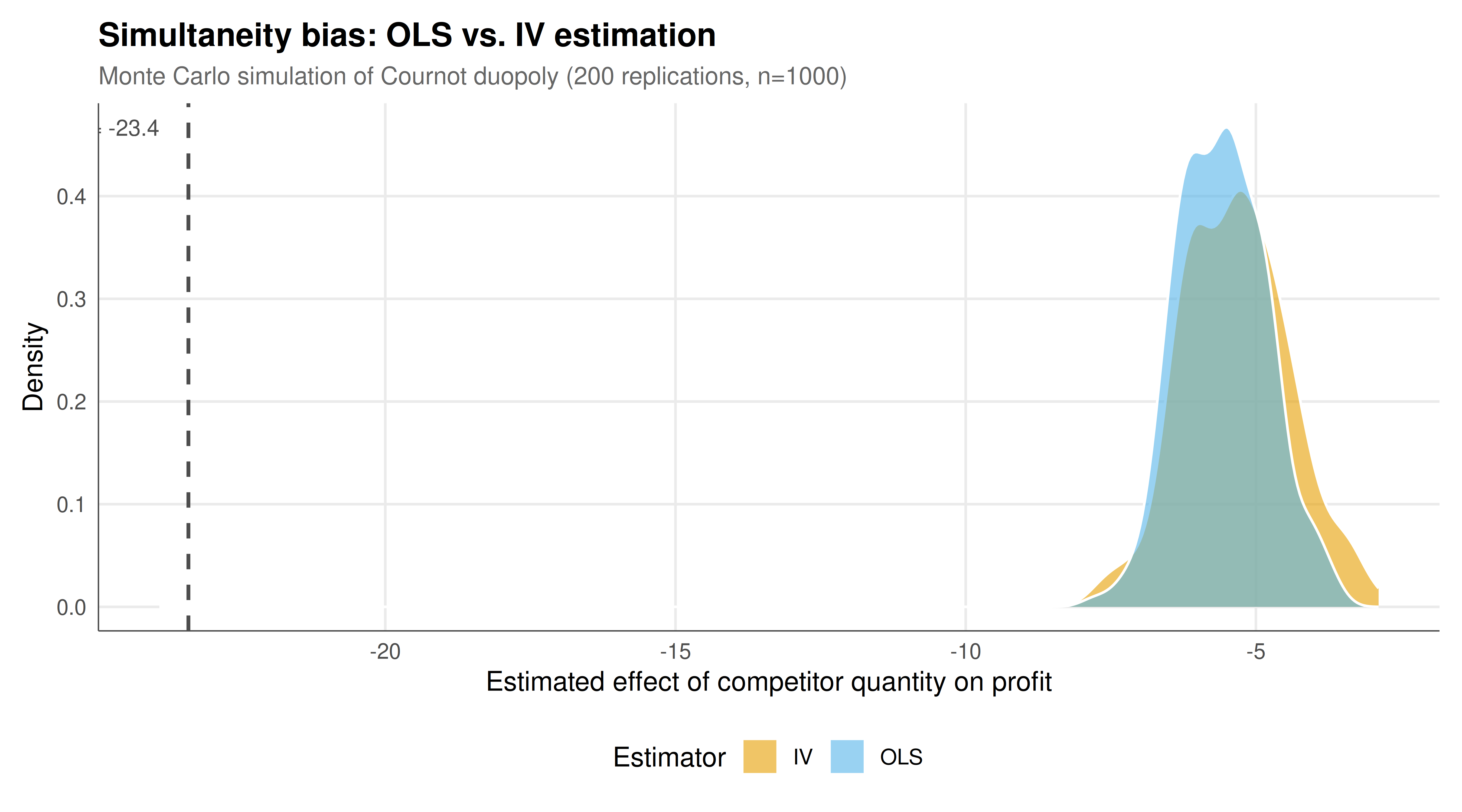
#| fig-cap: "Monte Carlo distribution of OLS and IV estimates of the causal effect of competitor quantity on firm profit across 200 simulations of a Cournot duopoly. The OLS estimator exhibits substantial upward bias due to simultaneity, while the IV estimator is centered near the true causal effect (dashed vertical line). Okabe-Ito palette."
#| dev: [png, pdf]
#| dpi: 300
#| fig-width: 9
#| fig-height: 5
p_static <- ggplot(mc_long, aes(x = estimate, fill = method)) +
  geom_density(alpha = 0.6, color = "white") +
  geom_vline(xintercept = true_effect, linetype = "dashed", color = "grey30",
             linewidth = 0.8) +
  annotate("text", x = true_effect - 0.5, y = Inf,
           label = sprintf("True effect = %.1f", true_effect),
           vjust = 2, hjust = 1, size = 3.5, color = "grey30") +
  scale_fill_manual(values = okabe_ito[1:2]) +
  labs(title = "Simultaneity bias: OLS vs. IV estimation",
       subtitle = "Monte Carlo simulation of Cournot duopoly (200 replications, n=1000)",
       x = "Estimated effect of competitor quantity on profit",
       y = "Density",
       fill = "Estimator") +
  theme_publication()

p_static
```
## Interactive figure
```{r}
#| label: fig-iv-interactive
#| fig-cap: "Interactive scatter plot of paired OLS and IV estimates from each Monte Carlo simulation. Hover over points to compare both estimates for the same simulated dataset. The dashed line indicates the true causal effect."
mc_scatter <- mc_results %>%
  mutate(text = paste0("Simulation: ", sim,
                       "\nOLS: ", round(OLS, 2),
                       "\nIV: ", round(IV, 2),
                       "\nTrue: ", round(true_effect, 2)))

p_int <- ggplot(mc_scatter, aes(x = OLS, y = IV, text = text)) +
  geom_point(alpha = 0.5, color = okabe_ito[1], size = 2) +
  geom_hline(yintercept = true_effect, linetype = "dashed", color = okabe_ito[3]) +
  geom_vline(xintercept = true_effect, linetype = "dashed", color = okabe_ito[3]) +
  geom_abline(slope = 1, intercept = 0, linetype = "dotted", color = "grey60") +
  labs(title = "OLS vs. IV estimates (paired by simulation)",
       x = "OLS estimate",
       y = "IV estimate") +
  theme_publication()

ggplotly(p_int, tooltip = "text") |>
  config(displaylogo = FALSE,
         modeBarButtonsToRemove = c("select2d", "lasso2d"))
```
## Interpretation
The Monte Carlo simulation provides a vivid illustration of simultaneity bias and the corrective power of instrumental variables in strategic settings. The OLS distribution is systematically shifted away from the true causal effect, confirming that naive regression of firm profit on competitor quantity produces biased and inconsistent estimates. The source of this bias is the equilibrium relationship: both firms' quantities are jointly determined by the common demand shock and the shared cost component, creating a spurious correlation between the competitor's quantity and the error term in the profit equation.
The direction of the OLS bias is informative about the underlying strategic structure. In our Cournot duopoly with a common cost component (the shared $\eta$ term), both firms face correlated cost shocks. When both firms experience a positive cost shock, both reduce output, and profits change in a complex way that confounds the direct competitive effect. The OLS estimator captures this confounded relationship rather than the pure causal effect of competitor quantity on profit. The bias is typically upward (toward zero or positive), attenuating the true negative competitive effect, because the common cost shock induces a positive correlation between $q_2$ and the unobserved factors affecting $\pi_1$.
The IV estimator, using firm 2's idiosyncratic cost shifter $z_2$ as an instrument, successfully isolates the exogenous variation in competitor quantity. The first-stage regression confirms that the instrument is relevant: the F-statistic substantially exceeds the conventional threshold of 10 for strong instruments. This relevance arises directly from the game structure -- firm 2's cost shifter affects firm 2's equilibrium quantity through its best-response function. The exclusion restriction is satisfied by construction: firm 2's idiosyncratic cost does not directly enter firm 1's profit function except through its effect on firm 2's quantity (and hence on the market price).
The IV distribution in the Monte Carlo simulations is centered near the true causal effect, confirming consistency of the 2SLS estimator. However, the IV distribution is notably wider than the OLS distribution, reflecting the well-known efficiency cost of IV estimation. By using only the exogenous variation in the endogenous regressor (rather than all variation), IV estimation discards information, leading to larger standard errors. This bias-variance trade-off is a central consideration in applied IV work: a biased but precise OLS estimate may be practically useful when the bias is small, while an unbiased but imprecise IV estimate may be less informative when the instrument is weak.
The weak instruments diagnostic deserves careful attention. When the first-stage F-statistic falls below 10, the IV estimator can exhibit severe finite-sample bias, sometimes worse than OLS. In our simulation, the instrument is strong because the cost shifter has a large direct effect on the firm's production decision. In real-world applications, finding strong instruments for strategic actions is often the binding constraint on credible causal inference. Researchers must rely on institutional knowledge of the game structure to identify variables that shift one player's best response without directly affecting the other player's payoff.
The broader methodological lesson is that game-theoretic structure and econometric identification are deeply intertwined. The same model that describes how players interact strategically also determines which variables can serve as valid instruments and how strong those instruments are. This complementarity suggests that empirical researchers studying strategic interactions should develop formal game-theoretic models not merely as theoretical exercises but as guides to identification strategy. Conversely, game theorists can benefit from understanding the econometric challenges their models create, designing models that are not only theoretically elegant but also empirically identifiable.
## Extensions and related tutorials
- [Surveillance and privacy as a strategic equilibrium](../../ethics-applications/surveillance-privacy-equilibrium/) -- an applied game where IV methods could identify the causal effect of surveillance intensity on compliance.
- [Von Neumann's minimax theorem](../../history-of-gt-mathematics/von-neumann-minimax-proof/) -- zero-sum game foundations that generate the strategic interactions creating simultaneity bias.
- [Multi-armed bandits and exploration-exploitation](../../ai-ml-foundations-and-applications/multi-armed-bandits-exploration/) -- causal inference connections through the exploration-exploitation framework.
- [Organ donation mechanism design](../../ethics-and-game-theory/organ-donation-mechanism/) -- mechanism evaluation where causal inference tools assess the impact of design changes.
## References
::: {#refs}
:::